1. Introduction (*)
Crop-climate interactions are of relevance for a number of applications, in food security, crop insurance, market planning and climate change impact assessments. All these fields have an interest in crop modelling and forecasting. The interest of forecasting goes beyond the immediate subjects discussed here, as all science is somehow about “forecasting”, i.e. based on my understanding of a system, I can make some guesses about how it will behave; the understanding can also be called “theory”, model or paradigm, and the system can be aso be called reality, a phenomenon or nature, for instance. Here I will focus more specifically on crop forecasting and the related data requirements.
A crop forecast is a statement that is made – before harvest – about the likely production (total amount of product expected) or the yield (amount of product/unit area, i.e. the intensity of production). Crop forecasts resort to some science (e.g. models and statistical methods) as well as a good amount of “art”, i.e. experience about approaches that do usually work, given the circumstances (type of crop, type of climate, local agricultural practices and available data). Crop forecasters are real-world people who stick their necks out. Take the following example: based on my forecast that the wheat production will exceed demand by 2 million tons, a government takes a decision to export the surprlus. If it is realised six months later that the surplus does not exist, and the government is forced to buy wheat internationally at a high price, they will certainly remember me!
In all cases, I need observations and data that are the basis of – or confort me in – my understanding, or my confidence that my understanding is correct.
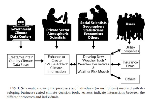
Source: D. Changnon & S.A Changnon, 2010.
The science of crop forecasting is relatively easy and straighforward, and relies on mostly well established methods from crop simulation to various fields of statistics1. The art is the difficult part. It has mostly to do with the way of blending empiricism and deficient data with the science proper, in such a way that it still results in useable and reasonably accurate forecasts.
Why “deficient” data? To start with because in most cases neither the locations the data are collected from, nor the type of data collected, and certainly not the policies of the agencies responsible for collecting the data, were designed for the specific purpose of crop forecasting. Indeed, even statistical methods used for calibrating crop models were designed to optimise statistical significance, not agronomic significance of agronomic applications2. All crop forecasting systems typically include a component dealing with data pre-processing and preparation which exceeds the crop modelling component in terms of time and methodological costs.
2. Data quality
Data are one of the components of decision making, but by no means the only one. Whenever data have to be used, and it is generally agreed that “good” data are a better basis for informed decision making.
One of the problems is that although it is a desirable feature for data to be “good”, there are no perfect data, and there is continuum between very reliable data and missing ones. The only real problem is to decide when data are “good enough” for a certain decision making process. It is suggested that the decision about “how good” data actually are cannot be decided based on the data themselves, but rather on the fruits of the tree, i.e. if the data and their processing produce a result which is useful for decision making, then the data are reasonably “good”.
Data used in crop forecasting can be classified in a number of different and inter-related ways.
3. From “probably good” to “probably bad” data
Data can be subjected to several well established types of quality checking, from the very obvious checks to the very sophisticated (Dahmen and Hall, 1990). “Internal checking” would include a comparison with extremes of the same element (temperatures with temperatures), and “external checking” would be, for instance a comparison of minimum temperature with dewpoint temperatures, or a comparison with data from a neighbouring stations (spatial check).
In a dataset recently downloaded from the NOAA WWW site, we find a file of monthly rainfall values, each with a flag indicating its “quality”, according to the following criteria:
- Flag 0: Passed the serial and spatial check
- Flag 1: Passed the serial and failed the spatial check
- Flag 2: Failed the serial and passed the spatial check
- Flag 3: Passed the serial check could not perform the spatial check
- Flag 4: Failed the serial check could not perform the spatial check
- Flag 5: Failed the serial and spatial check
- Flag 6: Missing (data not available)
Although the flags give the impression that we have a quality scale from 0 to 6, there is in fact no indication (nor does NOAA imply this) that it is more “important” to pass the serial check than the spatial check. Although one gets the feel that class 5 is worse than 1, there is no indication as to “how much” worse 5 is than 1 or 2. In practice, there is a category of the “bad” data which failed at least one test. By default, one has to assume that “good” data are the ones which failed all the tests to qualify as “bad” ones. In practice, it is almost impossible to decide how reliable or unreliable data actually are, but the recent report by Watts (2009) certainly confirms that the quality of no data can be taken for granted!

Take another example: “crop temperature”. In the earliest stages (seed and germination), the temperature a crop is exposed to is soil temperature, then it gradually becomes air temperature, until finally the actually temperature is the one created by the crop inside the field. There is thus an “effective crop temperature” which no thermometer or radiometer can measure.
Crop yield forecasts, at a highest level of integration, can but be regarded as semi-quantitative. Ideally, each individual forecast should be accompanied by an indication of the quality of the underlying data. Given the number and the variety of input parameters and data, a subjective statement of the “confidence” in the forecast is probably as close as we can get to assessing how “hard” the forecast actually is. In addition, we should not forget that all yield and crop forecasts are in fine calibrated against agricultural statistics. Strictly speaking, we thus forecast agricultural statistics, obviously not excluding their biases and errors. But then the decision making process needs “agricultural statistics equivalents”, and a forecasting method which would be so accurate as to produce data which are objectively more accurate than agricultural statistics would create a number of problems3.
5. Directly Measured data vs. “physically” or “statistically” estimated ones
Very few of the data used as inputs in crop forecasting are actually measured. Take rainfall: it can be derived from a number of sources, where raingauges constitute the only primary source. Radar estimates are calibrated against ground data, and so are the Cold Cloud Duration estimates used in tropical countries. This is a first source of error. A second source of error is linked with the spatial interpolations which are now normally carried out to spatialize the data. Here too, there are many techniques and no consensus about which to use, for what data, under which circumstances. In general, the data obtained indirectly are affected by sufficiently small errors and reasonably well know errors.
This applies mostly to physical data. When it comes to biological or agronomic variables (for instance crop planting dates), there is the additional complication that there is an inherent variability of management, a variability of the biological material (different varieties rather than the genetic variability of a given variety), and arguably a greater array of possible methods. For instance, planting date can be defined as the date/time when
- farmers actually plant, as reported from direct observation. This is the definition and thus also the “true” value;
- modelled soil moisture conditions become favourable;
- NDVI crosses a given threshold;
- the NDVI slope exceeds 0.04 units per dekad for more than 3 dekads;
- the sum of temperatures above a threshold of 3 degrees exceeds 153;
- more than 10% of mature wild apples have fallen off the trees;
- rainfall exceeds 53 mm in any 8 day period;
- the slope of the accumulated rainfall curve exceeds 3 mm/day for more than 9 days, provided that temperature does not drop below 11.7 degrees;
- etc, etc.
Obviously, all the “methods” above will yield correlated results which are spatially coherent (i.e they vary smoothly over space and do not give

One of the intermediate products used in the wheat time-series simulation shown in the figure above: wheat yield plotted against global radiation (estimated indirectly from rainfall!)
the impression that they vary randomly, unless some discontinuous variable -like WHC- has been used in their definition). It is very difficult to decide which method is best, and it is usually not very relevant either, provided a method is used consistently and the final yield function was calibrated with data obtained with the same method.
6. More about the “point data versus area-wide data”, spatial scale problems
The issue of the inter-compatibility and inter-comparability of point data vs. area-wide ones data is very frequently debated (Azzali, 1990; Hunt et al. 1991; Simard, 1991; Becker and Zhao-Liang, 1995). Some data are “native” point-data (P-data, like most weather data), while others (mostly satellite variables) are “native” area-wide ones (A-data). Again, as repeatedly indicated above the differences between the two categories are by no means so clear cut as might appear at first look. For instance radar rainfall: although it covers vast contiguous areas, the spatial resolution is so fine that it comes close to raingauge readings over short time periods4.
“Short time periods” are mentioned above because rainfall measured over longer time periods becomes representative for larger and larger areas. For instance, even in semi-arid tropical areas, there are good correlations between distant stations (100 km) if long enough time intervals are considered (months and above).
A lot of thinking was invested in the comparison of P-data and A-data, as well as A-data when the spatial resolution differs, for instance 1 km NDVI and 7 km NDVI. Depending on the way the A-data were calculated, the comparison of data at different scales is sometimes arduous. Similarly, the calibration of A-data with P-data (again, spatialization of rainfall is a good example) runs into difficulties which can be shown to be theoretical rather than only practical.
To illustrate this: there appears to be an upper limit to the coefficient of correlation between Cold Cloud Duration (CCD5) and rainfall in tropical countries. The actual variable of interest is the spatial average of rainfall over a given land area identified by a pixel, for which both CCD and the raingauge are only proxies. In addition, over short time periods, the raingauge gives information which is representative only for part of the pixel, while CCD, which is sampled at regular time intervals, provides a time-discontinuous estimate. It can be shown that in this specific example, the theoretical limit for the coefficient of correlation between CCD and raingauge is about 0.7 (Gommes, 1993). All this speaks very much in favour of aggregating data to a level which is well above pixel size!
More recent studies (e.g. by Beyene & Meissner, 2009) confirm that 15 years of scientific and technological progress (in terms of newer and more “powerful” satellites) did not substantially change the picture. In Ethiopia, values of r for correlations between satellite-determined and ground-based dekadal rainfall vary from -0.19 (winter) to 0.64 (summer, i.e. rainy season from May to October) for a spatial resolution of 8km. The study concludes that RFE [Rainfall Estimates] images can be used reliably for early warning systems in the country and to empower decision makers on the consequences caused by the changes in the magnitude, timing, duration, and frequency of rainfall deficits on different spatial and temporal scales. I read this differently: only 41% of rainfall variability (0.64 x 0.64 = 0.4096) is explained by the technique… and that’s not so much.
Three popular sources of rainfall estimates for Africa are illustrated below : FAO-RFE, FEWS/UGS-RFE and TAMSAT. Although there has been some technical progress since the days when rainfall was estimated by on 7 km METEOSAT cold cloud durations (CCD), such as smaller pixels and the integration of several products with METEOSAT imagery (Incl. ECMWF GCM for FAO-RFE), the issue of the fundamental incommensurability of raingauge and pixel remains .

There is a parallel of this scale question in time too. Some points linked with accumulating or averaging climate variables over longer time periods were mentioned above. In the specific case of crop forecasting, more or less complex variables derived from a crop model must be calibrated against actual yields. Time is built in as a regression variable, or yields are detrended, which leads to essentially comparable results. It is suggested that both cross-sectional6 and time series data can be used for the calibration, provided the areas covered are comparable from an agronomic point of view.
Two final points are to be mentioned in this section:
- the fact that many space-continuous data like soils can create artificial discontinuities in yield maps, if only because the real complexity (fractal structure ?) cannot be captured by ordinary maps at any scale;
- the fact that for many variables (WHC, soil water holding capacity), it simply does not make sense to treat them like A-data.7
The second point above is one of the main arguments against modelling crops on a regularly spaced grid. The alternative approach is to model at stations (where data tend to be more reliable) and then resort to some interpolation techniques which take into account the variations of a variable (like NDVI) which is reasonably well linked to yield.
Of course, there are contexts where the P-data are not even relevant, for instance for river basin simulation. Baier and Robertson have also shown that some variables (WHC) are so variable in practice, that the values computed using simple water balance methods are agronomically more meaningful!

Simulated correlation between satellite-based rainfall estimates by pixel and the amount of rainfall sampled by a raingauge, as a function of the distance between the pixel and the raingauge (km) and the cloud sampling frequency in munutes. The pixel size is assumed to be 7 km x 7 km. Details below under Gommes and Delmotte, 1993.
7. There are missing and “missing” data (8)
To start with, there are different categories of missing data. Many data termed “missing” are, in fact, “not relevant”. For instance, if no maize is cultivated in district A, both cultivated area and production are 0 (nil), but yield (production/area) is not relevant.
The example above also touches on the uneasy relations between 0 (nil) and “missing”, which may even creep into the physical data: “provisional” rainfall amounts are often used in water balance calculations, when dekads are used and the last day(s) have not been received yet. This leads to no serious consequence if amounts exceed soil storage capacity, and when the data bases are managed very carefully. This is, however, not always the case.
Still about the relation between 0 and “missing”: some values are so low, that they are “virtually 0”. For instance, only 250 Ha of sorghum are grown in province X as animal feed in Umbria. Should the sorghum yield from X be included in a calibration exercise? Probably not, as the area is in all likelihood marginal for sorghum and the yield is most likely to be an outlier. It would be better to consider that the area is actually 0. How low should the production figures be for the area to be considered “nil”? What are the criteria?
Technically, future data used in crop forecasting are also “missing”, and yet something has to be fed into the models.
8. About the reference averages to be used in crop monitoring
Farmers react very quickly to inter-annual fluctuations in weather, typically runs of wet years, runs of late springs etc. It is therefore indicated to take as recent and as short as possible a period as the reference for crop monitoring purposes. The five years preceding the current year would probably be ideal.
On the other hand climatologists recommend to use longer periods, preferably 30 years, as a reference value.
Depending on the inherent variability of the parameter to be used as a yardstick, the most recent period of about 10 to 15 years would probably satisfy both climatological and agrometeorological requirements.
9. Errors affecting forecasts
The errors which affect crop forecasts stem from a number of sources and causes, and it would be interesting to have a sensitivity analysis relating forecasting accuracy to the different sources of errors given below (Piper 1989; Cancellieri et al. 1993).
They include the following:
- observation errors in the primary input data;
- processing errors in the input data, including transmission and transcription;
- biases introduced by processing (statistical and other models errors), such as area averaging and the estimation of missing data, or the derivation of indirect measures (radar rainfall, radiation…). This also includes the effect of the somewhat arbitrary selection of one method rather than another (for instance gridding by inverse-distance weighting rather than kriging because IDW is less computer intensive, NOT because it is more accurate);
- “scale” errors, i.e. errors introduced by the fact that although some parameters are correct and meaningful when applied at a certain scale, they are used at different scales. This also applies to the time scale (for instance, instantaneous relative humidity has a meaning, but “average relative humidity” does not have any physical significance);
- errors in eco-physiological crop parameters;
- simulation model errors;
- errors due to factors not taken into account by the simulation model, for instance pests, or management decisions by farmers, or the weather at harvest;
- errors in the agricultural statistics used for the calibration;
- calibration errors, in particular less than optimal choice of statistical relation between crop model output and agricultural statistics;
- statistical errors in the “future data”, those used for climate between the time when the forecast is issued and the time of harvest;
- “second order” errors, those introduced by management decisions based on the early crop forecasts, or on the wrong interpretation of early forecasts;
- conflicts between results of different forecasts and forecasting techniques.
Number 12 may be a bit surprising, but in practice different techniques often yield conflicting results. Strictly speaking, this not affect the error on the individual forecasts, but certainly reduces the confidence the decision-maker can have in the data. What this points at is that the subjective confidence decision makers have in a method is probably more relevant the actual and objective error.
References, followed by Notes
(*) This post is based on the inputs prepared for Hough et al., 1998. See below. Also see this post, in particular this link.
Azzali,S. 1990. High and low resolution satellite images to monitor agricultural land. Report 18, The Winand staring centre Wageningen, Netherlands. 82 pp.
Baier,W. and Robertson,G.W. 1968. The performance of soil moisture estimates as compared with the direct use of climatological data for estimating crop yields. Agric. Meteorol., 5:17-31.
Beyene, E.G. & B. Meissner, 2009. Spatio-temporal analyses of correlation between NOAA satellite RFE and weather stations’ rainfall record in Ethiopia. Int. J. Applied Earth Obs. Geoinform., 12:69-75.
Becker, F. And Zhao-Liang Li. 1995. Surface temperature and emissivity at various scales: definition, measurement and related problems. Remote Sensing Rev. 2: 225-253.
Cancellieri,M.C.; Carfagna,E.; Narciso,G. and Ragni,P. 1993. Aspects of sensitivity analysis of a spectro-agro-meteorological yield forecasting model. Adv. Remote Sensing, 2(2-VI): 124-132.
Changnon & S.A Changnon, 2010. Major Growth in Some Business-Related Uses of Climate Information. J. Appl. Meteorol. Climatol., 49: 325-331
Dahmen,E.R. and Hall,M.J. 1990. Screening of hydrological data: tests for stationarity and
relative consistency. ILRI publication no. 49, WAGENINGEN, 58 pp.
Gommes,R. 1993. The integration of remote sensing and agrometeorology in FAO. Advances in Remote Sensing, 2(2-VI) 133-140. Click here for the text of the annex to the paper.
Gommes,R. 1996. Crops, weather and satellites: interfacing in the jungle. Pages 89-96 in: Dunkel,Z. (Editor), COST 77 Workshop on the use of remote sensing technique in agricultural meteorology practice, Budapest, Hungary, 19 and 20 September 1995. EUR 16924 EN, European Commission; COST Luxembourg, 289 pp.
Hough, M.N., R. Gommes, T. Keane and D. Rijks, 1998. Input weather data, pp. 31-55, in: D. Rijks, J.M. terres and P. Vossen (Eds), 1998. Agrometeorological applications for regional crop monitoring and production assessment, Official Publications of the EU,
EUR 17735, Luxembourg. 516 pp.
Hunt,E.R., Running,S.W. and Federer,C.A. 1991. Extrapolating plant water flow resistances and capacitances to regional scales. Agric. Forest Meteorol. 54(2-4): 169-196.
Piper,B.S. 1989. Sensitivity of Penman estimates of evaporation to errors in input data. Agric. Water management, 15: 279-300
Robertson,G.W. 1968. A biometeorological time scale for a cereal crop involving day and night temperatures and photoperiod. Int. J. Biomet., 12(3): 191-223.
Simard,A.J. 1991. Fire severity, changing scales, and how things hang together. Int. J. wildland fire. Volume 1(1): 23-34
Watts, A. 2009. Is the U.S. Surface Temperature Record Reliable? The Heartland Institude, Chicago, 31 pp. Downlodable from www.surfacestations.org.
1 The most efficient method to produce poor results is to regard crop forecasting as a data processing exercise rather than an agronomic one.
2 For instance, a crop forecasting method might want to minimize the relative error of a forecast, or the average absolute error rather than a “sum of squares of departures”.
3 If cost considerations are ignored, there is no reason why forecasts, if calibrated against field yields, could not be more accurate than agricultural statistics.
6 The “cross-sectional” data under consideration are yield statistics of several administrative units belonging to the same agrozone.
7 Maybe there is a need to develop concepts like “effective soil moisture”, the A-data equivalent of the purely P-type soil moisture. In the same way as “effective rainfall” is different from actually measured rainfall, there may be a way to define an “effective WHC” which, together with average area rainfall, average area ETP, “effective planting date”, etc would result in meaningful average area yield estimates. The same applies to phenology: it is sometimes more useful (convenient) to use a computed indicator than observed values (Robertson, 1968).
8 This section is mostly taken from Gommes, 1996. The quoted paper has an additional note which does not apply to the European Union, but there may be parallel situations in other temperate countries. Missing data sometimes carry at least as much information as actual ones. One of the best examples can be taken from the field of marketing: prices sometimes keep rising for weeks, due to short supply, until the commodity eventually disappears from the market. The data item information, in that case, is technically missing, but it remains very relevant and paradoxically carries a lot of useful information. A parallel example can be taken in the field of demography: human populations temporarily or permanently migrate out of the villages in the case of very serious food crises. Is the population now “nil”, missing or “not relevant” ? This example clearly shows the importance of the spatial and temporal aspects..