This post of part of a set of three. The current What is “abnormal” weather? is the main one, with two ancillary ones dealing with the issues of Trends in climatological time series and The statistical distribution of some climate variables.

A silence follows, then Dr Michaels says: But you are looking to judge what is abnormal? Dr Frankl: To be honest, we are not really interested in such terminology because that word is theoretically unclear and practically it does not help us. Alice Jolly, The Matchbox Girl, 2025. Bloomsbury, 416pp.
This post is, somehow, about “Science” Vs. “Common sense”. It is about the reference values traditionally used by some climatologists and institutions to define normal weather1 conditions. This is not a simple subject, because the words “normal”, “average” or “expected” are roughly equivalent in everyday language, but not in the jargon of meteorologists and climatologists. This is a subtlety that many users, including some who crucially depend on weather for their livelihoods, such as the farming community, do not necessarily perceive to a sufficient extent.
In a nutshell: the tradition is to use a 30-year average of weather variables (e.g. rainfall, temperature) during the recent past and consider this to be the “normal”. My point is that, during a period when weather consistently changes fast from year to year, the average is meaningless if weather displays a trend, as with the current warming period2. Since not all weather variables are affected in the same way by the ongoing changes, this post applies to different degrees to different weather variables3, as will indeed be illustrated below for rainfall and temperature using data from Uccle, Belgium.
My point is also, specifically, that we are in a period where many things appear to be changing across the spectrum of human experiences. The changes themselves, their magnitude, causes, inter-connectedness, severity etc are all open to debate, and their perception contains an element of subjectivity. But what I most I dislike and fear is the gentle hum of our intellectual routines when it makes the world more dangerous.
Defining a climatological normal
Let’s have a closer look at the concept of “climatological normal” as used by National meteorological services – often referred to as NHMS (National Hydrological and Meteorological Services) – which strictly adhere to the recommendations of the World Meteorological Organization, WMO3. Here is a quote from WMOs standard reference document Guide to climatological practices (WMO 2018)4: Climate normals are used for two principal purposes. They serve as a benchmark against which recent or current observations can be compared, including providing a basis for many anomaly-based5 climate datasets (for example, global mean temperatures). They are also widely used, implicitly or explicitly, to predict the conditions most likely to be experienced in a given location. The document further explains that the standard normals are computed over 30 year periods and that those 30 years are themselves standard, essentially every 10 years for 30-year periods at the start of every decade from the year ending with digit 1 (1981–2010, 1991–2020, etc.). This is because 1981–2010 normals would be viewed by many users as more “current” than 1961–1990 among others because there is also a need for more frequent calculations of climatic normals in a changing climate.
The text below is subdivided into two main sections: (1) an assessment of the use of the 30-year period in practice and (2) an illustration using data taken from the Belgian agrometeorological bulletin.
(1) Why climatological normals are often dangerously misleading
There are several unrelated reasons why 30-year averages may not represent “normal”, “average” or “expected” conditions under climate change conditions.
An important point to realise about the statisticians’ 30-year period is assumed to represent a sample of 30 observations (N=30) drawn from a much larger pool (set) of data which represents the actual population. It is thus obvious that our sample has limited variability compared with the actual population. Statisticians may imagine that they can draw as many 30-year samples as they like from the actual population, but climatologists cannot: they sample one year at a time as the time passes… More or less by definition, the actual variability of past climate/weather underestimates the potential variability. In other words, with or without climate change, there will be “surprises”, i.e. an “extreme event” that has never happened before4. Refer to note 8 in this other post for a discussion about the the normality – or the absence thereof – of climatic data.
| Allow me insist that there is no magic and little “science” involved in defining the number of years (i.e. N=30) that make up the period that defines a climatological normal. Climatologists have borrowed the concept from statisticians, who are often very practical and non-dogmatic people5 confronted with very down-to-earth issues. “30” in statistics is not unlike “7” in “the seven colours of the rainbow”, the “seven seals”, the “seven dwarves”, the “seven seas” and the “seven continents”. One can indeed see 7 colours in a rainbow, but nothing prevents anyone from counting 11. 30 means “sufficiently large but not unmanageable”. There is nothing rational about it. So, why 30 you may ask? (Sharma, 2020.) |
In practice the knowledge about the statistical normality of climatological data loses a lot of relevance when considering other features of the data, in particular (1.) the possible presence of trends and (2.) symmetry – or the absence thereof – of the climatological data’s distribution.
- If weather observations of the previous seasons follow a persistent trend, the current weather will, in all likelihood, be akin the weather of the recent years recent, and certainly not like the weather that prevailed 30 years ago. As illustrated in a separate post on Trends in climatological time series the 30-year period, however, often leads to inconclusive significance issues.
- A more subtle issue has to do with the statistical distribution of individual variables, especially rainfall. Unless an un-trended variable follows a well-behaved (and rather theoretical) symmetric, preferably bell-shaped distribution, “average”, “normal” and “expected” will be different. I had initially planned to explain this issue in a foot note, but the subject is too complex for a foot note. I eventually wrote a full post on the subject. What this boils down to is that the average value of most climatological variable time series is rarely the expected value.
- The third reason why climatological normals or 30-year averages are to be distrusted is that many weather-dependant activities, especially farming, have reaction times that are much faster than 30 years. If a maize crop has failed five years in a row because of drought, a farmer will not take the risk of 5 more failures. Instead, he’ll start diversifying out of maize immediately6.
(2) An illustration based on Belgian data
Winter climate at Uccle according to the bulletin of the Belgian Crop Growth Monitoring system
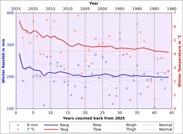
This discussion is based essentially on Figure 1, a rather “rich” graph7 published in the May 2025 bulletin of the Belgian Crop Growth Monitoring system. All bulletins are available in French and in Dutch. Figure 1 illustrates data belonging to the station of Uccle (50.796862 N, 4.357871 E, Altitude 100 m), the location of the headquarters of the Belgian meteorological service; it is part from the Brussels conurbation and located about 15 km from the nearest agricultural area.
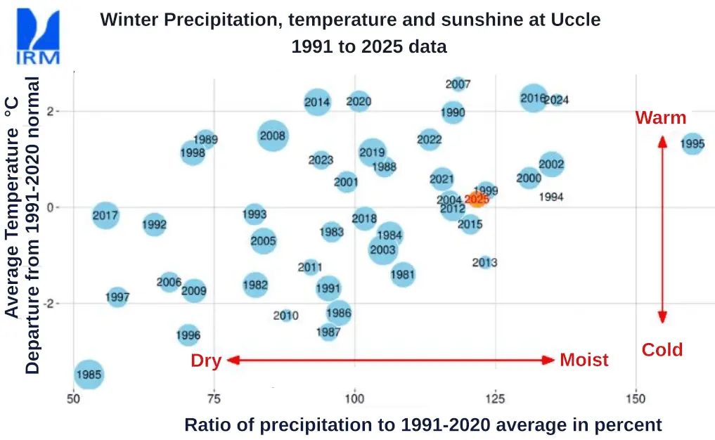
For the purpose of the analyses below, it was assumed that “winter” includes the time period from the 3rd dekad8 of December (21 to 31 December; dekad 36) to the second dekad of March (11-20 March; dekad 8). Average climate data for a slightly different period (1991-2021) were obtained from this source. In order to compute whole winter data (dekads 36 through 8) it was necessary to first obtain dekadal values corresponding to dekads 36, 7 and 8 (the last dekad of December to the two first dekads of March. Dekad values were interpolated from monthly values using the method described in the Footnote9. The average 1991-2021 winter temperature was found to amount to 4.2°C and the precipitation total to 198.7 mm. From there, it is possible to estimate the absolute values corresponding to Figure 1.
How did Uccle winter weather data change over time?
Figure 2 and Table 1 shows basically the same data as in Figure 1, using absolute values of the variables instead of relative ones. It is immediately apparent that the data are affected by trends, as happens for most recent European climate data. How meaningful are those trends?
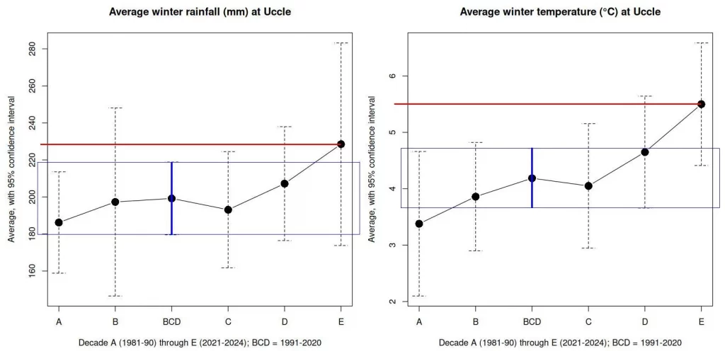
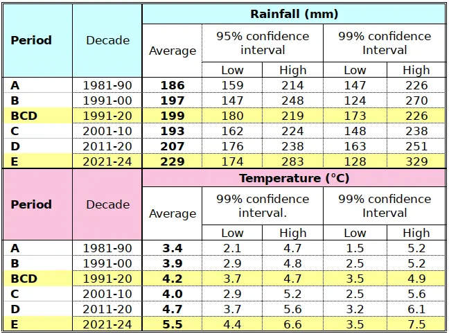
Since 1981, rainfall values increased by about 23% on average (period A to period E). There has been a “constant” trend towards higher rainfall but with a considerable amount of variability. For instance, the 99% confidence interval for the 1991-2000 average ranges from 124 to 270 mm, with the highest recorded rainfall in 1995 (Figure 1). The recent 4-year average (2021-2024) at 228.5 does not . The latest average (228.5 mm) does not fall within the 95% confidence interval of the 1991-2020 mean, but just makes it for the 99% interval of 173 mm to 226 mm. Altogether, the 1981-2024 rainfall trend is weak.
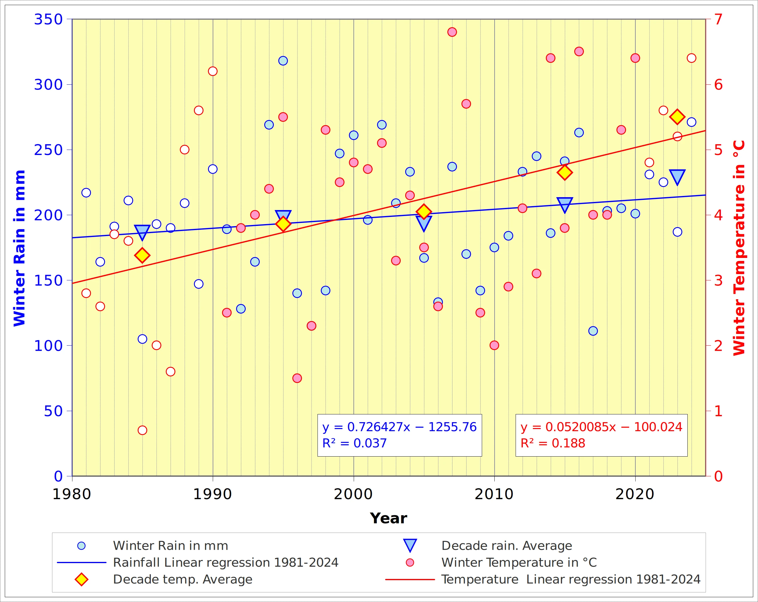
Temperature variations over time are generally more pronounced than rainfall variations, in the sense that there has been a steady increase from 1981, with a marked acceleration in recent years (Table 1: 3.4°C, 3.9°C, 4.0°C, 4.7°C and 5.5°C, respectively for the successive decades). Figure 3 displays all historical values from 1981 together with the corresponding linear trend lines. The critical Values for Pearson’s Correlation Coefficient for 42 degrees of freedom (d.f.) are 0.2973 at the 0.05 threshold and 0.3843 at the 0.01 level. It appears that the trend is not significant for rainfall (R=0.19; R²=0.037) but highly significant for temperature (R=0.43; R²=0.188). If we restrict the trend calculation to the “normal period” (1991-2020, d.f.=28) then the coefficients of correlation are 0.0357 and 0.2702 for rainfall and temperature, respectively. With the threshold values of R=0.3610 (P=0.05) and R=0.4629 (P=0.01) none of the trends is significant. Finally, if we include the last 30 years on record (1995-2024), the coefficients become 0.0854 for rainfall and 0.3505 for temperature. They are still not significant, even if temperature “almost makes it” (0.3505 Vs. 0.3610) at P=0.05.
An alternative reference period to the 30 year “normal”
Regardless of the significance issues underlined above for trends, it does make sense to adopt a reference period that is different from the “normal”. For temperature, the Uccle “normal” lacks the stationnarity of the mean criterion and, therefore, does not qualify. For rainfall, however, the absence of a significant trend, the 1991 to 2020 is acceptable. The main issue, in this case, is to know whether the rainfall distribution is reasonably symmetric. Based on this post, the option cannot be excluded and will not be pursued in detail here.
Between 1981 and 2017, the rainfall averages computed back from 2024 insignificantly depart from the 1991-2020 average. Together with 1985 and 1997, 2017 was one of the driest years of the period of interest (Figure 1). After 2017, the short-term rainfall increased constantly: 1 year ” average” (2024), 2 years (2024, 2023)… 8 years (2024 through 2017) but the variability was such that the 1991-2020 average stays with the current confidence interval. As mentioned in Trends in climatological time series and above, there is no particular reason to contest the validity of the normal as a reference.
Temperature, however, is different. The recent averages tend to be systematically higher than the 1991-2020 normal, and the increasing trend has been visible from the 198011 . From about 2011, the 1991-2020 normal is no longer included in the confidence envelope of the back-computed average.
Concluding remarks
There is ample evidence in Uccle average winter temperatures that the standard “normal” (1991-2020 30-year average) has been gradually loosing it’s relevance as a reference. For rainfall, the conclusions are less clear. There are several good reasons why 30 years are currently inadequate to define reference climatology, and this includes (1) the sheer arbitrariness of the 30-year period, (2) the fact that averages are not meaningful in trended time series and (3) the period is far too long for decision making, in particular in farming. It is suggested that a reference period not exceeding 15 years (maybe 12, or 10?) would be much more meaningful for agricultural ” tactical” (i.e. year-to-year) decision making.
Incidentally, and this is no coincidence, even in a situation where the statistics are inconclusive (e.g. normality and trend concerning rainfall in Uccle), a shorter reference period would not have a negative impact on the relevance of decisions taken compared to a longer period. A final point: using fixed reference periods (e.g. 2011-2020) may be easier to handle when averages are re-calculated by hand, but this is no longer justified when a computer puts out calculations results in seconds. Shifting reference periods (e.g. the 12 previous years ending last year!) are more meaningful than fixed ones!
Some relevant references12
Alexander L V 2016 Global observed long-term changes in temperature and precipitation extremes: A review of progress and limitations in IPCC assessments and beyond. Weather and Climate Extremes 11:4-16.https://www.sciencedirect.com/science/article/pii/S2212094715300414
Arguez A, Vose R S 2011 The Key to Deriving Alternative Climate normals. Bulletin of the Americam Meteorological Society, 699-704. https://journals.ametsoc.org/view/journals/bams/92/6/2010bams2955_1.pdf
Bari D 2021 Concept of and Calculation of Climatological Standard Normals for 1991-2020. WMO Web document: https://dgm-meteo.github.io/w-cdmse/Docs/DGM-OMM-CLINO-EN.pdf
Faures J M, Bernardi M, Gommes R 2010 There is no such thing as an average: how farmers
manage uncertainty related to climate and other factors. Water Res. Dev., 26(4):523–542. Full text.
Gommes R 1983 Pocket computers in agrometeorology. FAO Plant production and protection
paper N. 45, FAO, Rome, 140 pages.
Sharma A 2020 Is n = 30 really enough? A popular inductive fallacy among data analysts. Ruminating Verbose of Statistics Part I. Blogpost: https://towardsdatascience.com/is-n-30-really-enough-a-popular-inductive-fallacy-among-data-analysts-95661669dd98/
Trewin B C 2007 The Role of Climatological Normals in a Changing Climate. Edited by Omar Baddour and Hama Kontongomde, World Climate Data Monitoring Programme Series WCDMP-No. 61. WMO-TD No. 1377. WMO, Geneva. 45 pp. https://www.uncclearn.org/wp-content/uploads/library/wmo46.pdf
WMO 2018 Guide to climatological practices. WMO-100. WMO, Geneva. 141 pp. http://wxdata.metoffice.gov.ag/intranet/WMO_docs/WMO%20No.%20100%20Guide%20to%20Climatological%20Practices%20-2018.pdf
WMO 2025 State of global climate 2024. WMO-1368, 37 pp. Geneva. https://library.wmo.int/viewer/69455/download?file=WMO-1368-2024_en.pdf&type=pdf&navigator=1
Notes
- It is not always obvious whether one should say “weather” or “climate”. Weather is defined by the atmospheric conditions as they happen. It is raining: the weather is rainy. It is freezing: the weather is cold, or maybe cold and windy etc. The conditions we are exposed to at any moment is weather. Like the speed indicated by a car speedometer, it is an instantaneous value. When weather is recorded over a longer time period, we can define “normal”, “average” or “expected” weather, which is defined as climate. When I say that dzuds frequently occur in Mongolia during winter, or that haboobs will mostly befall Arizona during July and August, I am making climatological statements. Climate, like average speed, expresses a more synthetic, summarizing value. Climate is defined statistically as the average (i.e. the arithmetic mean) of weather, i.e. the variables that characterize climate are the averages of the corresponding variables (rainfall amount, windspeed…) that characterize weather. Variability patterns are part of the definition of climate. ↩︎
- We read last January that, according to WMO, 2024 was the warmest year on record at about 1.55°C above the pre-industrial level. But there is more: the State of global climate 2024 report (WMO, 2025) tells us that the ten years from 2015 to 2024 were individually the ten warmest years on record. Can we say that 2024 conditions were abnormal? This a point that can be debated ad infinitum. 2024 conditions were abnormal compared with, say, the 1950s, but the warm 2024 was certainly not a surprise. Nor will 2025 be, as we know from current observations show that the warming trend continued this year. This was confirmed by Copernicus… month after month. ↩︎
- Many people refer to “weather parameters”. The word “parameter” is wrong. It is even worse than “normal” when considering its different meanings. A “parameter” is a setting. When we refer to observed weather or climate, the best word to use is “variable”. My post on Crop monitoring dialects has a short discussion on the terms index, indicator, variable, parameter, factor, element, descriptor and metric. ↩︎
- There is a technique known as Random weather generators (RWG) or more correctly Stochastic Weather Generators (SWG). SWGs are software programmes that produce synthetic (artificial) time series of realistic-looking weather/climate data, each of which is a sample drawn from a supposedly infinite pool of data. This can be very sophisticated in practice, when the generated data maintain realistic inter-correlations and even spatial coherence. “Realistic inter-correlations” means that, for instance, temperature and sunshine will be low during rainy episodes, as happens in the real world. Spatial coherence means that areas that are geographically close will be assigned similar values. In this way, if I am interested in assessing climate change impact on some human activity (say crop production), I can generate with a SWG 10000 possible future scenarios and use each of them to estimate the future crop production between now and 2050. One of the problems is that the SWG was “trained” with historical data and that it will generate synthetic data that are “compatible” with the historical data, i.e. basically the same variability patterns. Variability can be parametrised but this parametrization contains some element of arbitrariness. If there is a trend in variability, I can, to some extent, extrapolate the variabilty into the future. ↩︎
- For instance, the fact that people often have to work with very small samples (e.g. N=10). Also remember that many statistical methods have been invented by non-statisticians. Bayes, for instance, was a Presbyterian minister. Gossett, of student’s t fame, was a chemist and brewer. Fisher, the inventer of ANOVA, was an evolutionary biologist. There are many more examples (e.g. Neural networks) that show that statistical invention was often fathered by necessity! ↩︎
- This is a complex issue, as there are often non-indifferent financial issues to be considered. The transition from a production system to a another can take 5 to 10 years. This is a period of increased vulnerability and farm insurances should build this into their risks portfolios if they want to promote less risky farming. What I observe here in Piemonte (Italy) , is a replacement of low quality wine production by hazelnuts, which Ferrero will buy. People aiming at, and succeeding in high quality wine production do not need to diversify into hazelnuts. Hazelnuts are a risky business which, in my view, has not been correctly assessed. The risks patterns are directly under the influence of high weather variability and susceptibility to drought impact, high pesticide use, and irrigation using non-renewable water. ↩︎
- “Rich” in the sense that it condenses a lot of information. ↩︎
- A dekad (spelled with k) is a ten-day period used in agrometeorology and climatology, when an operational length of time shorter than a month is required. The term was originally recommended by the (now defunct) WMO Commission for Agricultural Meteorology to avoid the confusion with “decade” which has come to mean “10 years” in English. Other languages (e.g. French) more logically refer to decennia (or decenniums, 10 years) and decades (10 days). ↩︎
- Rainfall values (or other sums) for the third dekad of the months (D3) are obtained from the values of the previous, current and next months (C1, C2, C3) as D3=(-4C1+26C2+5C3)/81. For temperatures (or other averages), the first and second dekad values are computed as D1=(5C1+26C2-4C3)/27 and D2=(-C1+29C2-C3)/27. The derivation of the formulae can be found in a very old publication of mine (Gommes, 1983) of which the relevant chapter is available here. ↩︎
- The graphs in figure 2 were prepared with R and the Gnumeric function confidence.t was used to estimate the confidence intervals. ↩︎
- It is assumed this is a genuine warming effect. Since the station is in an urban context, urbanization per se does not seem to be an issue. There have been , however, changes in the measuring technology and minor location shifts of the instruments. Maybe the Belgian meteorological Service has done some studies on the subject? ↩︎
- Not all are quoted in the text. ↩︎