When they have been in a business long enough, “experts” often develop a gusto for the more philosophical side of their trade, and crop forecasters are no exception. Strictly speaking, the philosophical aspects are not needed to build a forecasting method. They are, nevertheless, very useful to avoid naive errors that can result from applying technical methods without paying too much attention to the overall context. So here come some of my personal “crop yield forecasting rules.” (First published: 20140727 / Last Updated: 20141018)
Rule 1: crop yield forecasting is art as much as science
This fist rule expresses the fact that different people will derive different solutions based on the same data, and some will be demonstrably better than others: Easier to use, less data hungry, more accurate and repeatable. There is, of course, a lot of “science” in crop yield forecasting, but the science is the servant of the forecaster, not his master. Some people behave as if the tools were the master: typically remote sensing, or multiple regression. A crop forecast is not a data processing, statistical, remote sensing or a GIS problem. It is an agronomic/agricultural problem!
Even if you are not an expert in agriculture, and you find some rainfall data, you will get good correlations between national millet yield in Niger and total national annual rainfall accumulation averaged over all weather stations (which is the kind of things some people do!). But if you try the same with sunflower in Europe, you are in for a headache. Some forecasts can be improvised, but most cannot.
Rule 2: If statistics contradict agronomy, blame statistics; if common sense contradicts agronomy, blame yourself
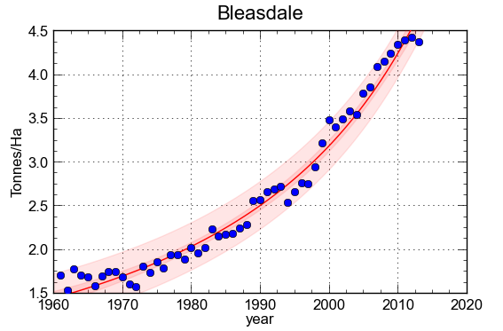
Total rice yield (as tonnes of paddy/Ha) in Bangladesh since 1961. The yield was modelled using a Bleasdale equation (a+bx)^(-1/c). The coefficient of determination is 0.979 and the average error on the yield is +0.13% while the average absolute error is 4.5%; both values are more than acceptable by all crop forecasting standards. The coefficient of determination means that only (1-0.979)*100= 2.1% of the variability – at the national level – is accounted for by non-trend factors. Every attempt to “explain” the 2.1% by weather or other factors is self-defeating. Based on the trend, the 2014 yield would be estimated at 4.87 tonnes/Ha. It is stressed that rice farming in Bangladesh is extremely complex, with very high cropping intensities close to 200%. The average shown is thus the result of three different crops, including a dry season irrigated crop known as “Boro.” At a different scale, for instance at the district level and for a single crop (e.g. only Boro) modelling becomes meaningful because as little as 10% of variability is accounted for by the trend. Graphs based on FAOSTAT data analysed with CurveExpert.
The tendency is to take a heap of yield data and weather data (they are “factors”) and remote sensing data (they are not “factors” in the sense that they do not affect yield, they are “descriptors”) and then start regressing and keep whatever comes out of the process. There is usually no attempt to “understand” the data by identifying significant factors, and there is no elementary verification, such as cutting the training (calibration) data into two random or chronological batches, and verifying that similar coefficients are obtained. The result is that, as I have seen in a large Asian country years ago, practitioners sometimes get negative coefficients for sunshine’s contribution to irrigated rice. And that’s wrong. I need no checking of any kind: it’s wrong. The statistics are to blame – or the data – but thourough re-checking is needed in any case… which takes me to the common sense part of the heading.
If the statistical work was done correctly and honestly, and you still cannot get a decent yield estimate, the problem has deeper roots, which are most interesting (and useful!) to uncover. Maybe the data have a technology trend that was not taken into account? Maybe the data are not variable enough? If the variability (in terms of coefficient of variation) is just a couple of %, there is little to explain, actually. In Bangladesh, total rice output cannot be forecast using environmental factors, because the total variability is just a couple of percent. If half of it is due to weather (and the other half to other factors such as weeds, management, diseases, pests), trying to model it is self defeating. This is why the agrometeorologist-artist also has to know when to throw in the towel!
Rule 3: All crop forecasting is statistical
Even if you use a simulation model (also known as analytical model, or process -oriented model, note 1) it will need adjusting statistically in the end in order to get realistic yields. This is, actually, one of my preferred approaches, next to “non-parameric forecasting” (note 2): you run a model, and use model state/auxiliary variables (including modelled “yield” ) as inputs in a statistical model. I call such variables “agronomic value added variables” because they are an agronomic interpretation of the above-mentioned factors and descriptors. Another reason why “all models are statistical models” is that we are usually interested in regional forecasting (=district, or regional forecasts), a scale at which the inputs and parameters used to tune process-oriented models (= simulation models, = analytical models) are just meaningless, because such models were designed to operate at the level of a field.
The three “rules” above are my basic “rules”. I have more, but the ones above are findemental. I also have the “twelve sources of errors” in yield forecasting… because there are many different ways of getting a forecast wrong, some of them “second order.” Imagine you are a forecaster with a good record, and that you are specialised in oil palm. Most palms (including coconuts and oil palm) develop their fruits over three years, which sometimes leads to very early forecasts. If you forecast at the beginning of year three that there will be an over-production of palm oil, plantation owners will be tempted to reduce costly inputs. As a result, your forecast will be wrong… because it was correct in the first place!
Someone should definitely write a good practical book about crop forecasting! As an appetizer, look up this little book by Balaghi et al. (note 3, for some handy references), which is an excellent illustration of the rules above: a crop forecaster must know her tools to start with, but first of all she must now her crops. The booklet is about Morocco, but the philosophy of the approach is a lesson that can be applied everywhere.
Notes
Note 1: Here is a list of some of the popular simulation models. Click on the name to be directed to the model’s home page. There is, currently, no good and simple model designed for the regional scale, although there are several downgraded versions of the models below. These are not, however, an acceptable substitute for a model specifically designed for regional applications.
- WOFOST (WOrldFOodSTudies), Wageningen Agricultural University, C.T. de Wit and followers, originally designed for food security studies. A very large family of models: they even have one for tulips.
- CropSyst (Cropping Systems Simulation Model), WSU, Claudio Stöckle, a good simple multi-purpose model
- AquaCrop, FAO, Dirk Raes (UC Leuven) and Pasquale Steduto (FAO), originally developed for farm-level irrigation planning, but the model is gradually developing into something less and less appealing… because it is so difficult resisting the temptation to build in more and more functions.
- DSSAT/CERES, Decision Support System for Agrotechnology Transfer/Crop Environment Resource Synthesis, optimimize farm management & crop rotations at farmers’ level, Gerrit Hoogenboom/Gordon Tsuji, U. Georgia/Hawaii. One of the most sophisticated (= heaviest) models around. Never used for real world forecasting because inputs are just meaningless at the regional scale.
- EPIC (Environmental Policy Integrated Climate), Texas A&M, Jimmy Williams, originally a tool to assess the impact of farming on erosion, but has developed into a big multipurpose tool.
- APSIM, Agricultural Production Systems Simulator, very ambitious simulator of complete agricultural systems, mostly sponsored by CSIRO, the State of Queensland and the University of Queensland in Australia. Very likable family of models because they are less “commercial” than some of the others above, and even use R for some modules!
Note 2: “Non-parametric forecasting” is a mostly analogical procedure where the current cropping season (the yield of which is to be forecast) is compared with previous seasons in order to identify similarities: “this year is a year like 2008, and we expect a yield like the one we had in 2008!” The reason why this works is actually not so obvious, and is related to the fact that environmental variables are correlated over time, over space and among them (cloudiness with temperature etc.) See this paper: Gommes, R. 2007. Non-parametric crop yield forecasting, a didactic case study for Zimbabwe. ISPRS Archives XXXVI-8/W48 Workshop proceedings: Remote sensing support to crop yield forecast and area estimates, 30 Nov. – 1 Dec. 2006, Stresa, Italy, p. 79-84. Click here to download it.
Note 3: Here is the reference to the book by Balaghi and his colleagues: Agrometeorological Cereal Yield Forecasting in Morocco, by Riad Balaghi, Mohammed Jlibene, Bernard Tychon and Herman Eerens, 2013. Published by Institut National de la Recherche Agronomique du Maroc, ISBN: 978-9954-0-6683-6. 157 pages. It can be downloaded from here. A French language version is also available. Readers may also be interested in a generic introduction by Gommes et al.: Gommes, R., H. Das, L. Mariani, A. Challinor, B. Tychon, R. Balaghi and M.A.A. Dawod, 2010. Agrometeorological Forecasting. Chapter 6 of WMO Guide to Agrometeorological Practices (GAMP), WMO N. 134, Geneva. 49 pp. The publication is available from the official GAMP website (click here); an earlier and better version (though not so nicely formatted!) can be downloaded from the website of the International Society of Agrometeorology.
Dear René,
Thank you very much for your efforts to popularize the agro-meteorological science. What I’m going to write, is not directly related to the rules that you just mentioned but it must be said to the adventurers who want to engage in predicting crop yields. In general, whatever the prediction you make at the country level, there are few people who can contradict you because nobody has reasonable means to achieve a comprehensive assessment. You will also note that the figures you provide do not make policy makers happy. You will also notice that the quality of your predicted yields will be swallowed up by the enormity of the area estimation error, so that ultimately the production figures will have no relationship with your work. Conclusion: arm yourself with your skill and patience to fight against the skeptics and politicians, even with the best science in the world. But ultimately, they will recognize your skills through your methodological approach. The three rules of René Gommes are a very good start for beginners and not so beginners.
Riad
Many thanks, Riad, for the comments and for being my most faithful reader! You are quire right, actually. Maybe the first rule should be “Be patient with all your customers and keep trying”.
Very useful insights concerning the crop forecast science (and indeed…art).
Also the book Agrometeorological Cereal Yield Forecasting in Morocco
Best Regards