Routine crop monitoring is done with indices which indirectly describe or capture the effect of environmental variables on crop condition and yield. Among the indicators that indirectly “capture” crop condition, NDVI is certainly one of the most popular and most easily available from a variety of sources. The word “indirectly” refers to the fact that, depending on pixel size, NDVI includes a mix of crop and natural vegetation and the practitioners of crop monitoring usually consider that the factors that affect crops do affect natural vegetation in a similar way, so that NDVI provides a good quantitative or semi-quantitative indicator of crop condition. See, for example, the following websites for typical examples: EC/MARS, USDA/FAS, FAO/GIEWS and CropWatch, to mention only the major international systems.

Recently, CropWatch has published a bulletin where an old biomass indicator (the “Miami” NPP potential) was used as a monitoring tool, with rather interesting results, as it assesses the combined effect of two important crop production factors (as opposed to descriptors such as NDVI). It was found, however, that NDVI-based indicators and Miami NPP efficiently complement each other.

The original Miami NPP (more details below) is based on total annual rainfall and average annual temperature data from meteorological stations. Strictly, it should thus be used only for monitoring complete seasons. The present post examines to what extent the method can be used for monitoring shorter periods (groups of dekads). Althouh the description below refers mostly to ground-based (station) data, the CropWatch implementation was based on a  combination of satellite-derived rainfall and temperature.

The standard Miami NPP described

In the mid 1960s and seventies, after decolonization, countries where rediscovering the global dimension of the world; international organizations launched studies aiming at assessing the production potential of the planet, including natural vegetation (Unesco), crops (FAO’s Agroecological zones project; FAO 1978-81, FAO 1980) and soils (the FAO/Unesco soil map of the world). This is also the period when the Club of Rome published Limits to Growth, another study aiming at matching resources availability and requirements and which was to become the first of a long series of similar studies and scenarios published over the last 40 years (Meadows et al, 1972).

This was also a time when computing power was still limited and when plant and crop simulation models where still very much confined to the academic world, especially the pioneering “school of Wageningen” in the Netherlands developed around CT de Wit (de Wit et al 1972, Bouwman et at 1996). As a result, relating environmental factors to biological production potentials was still assessed mainly using empirical equations, such as the Miami model of Helmut Lieth (1972, 1973).

Lieth proposed the following equations, which constitute the basic Miami model. They are referred in this context as NPP_1: NPP based on annual climate variables for year y, Rain(y) and Temp(y), the total annual rainfall (mm) and the annual average temperature (deg. C)

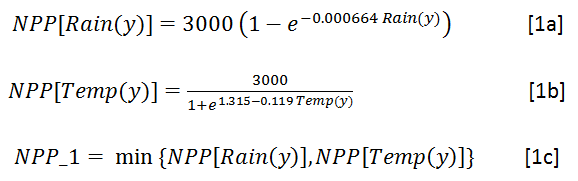
with NPP_1 expressed in grammes of dry matter per square meter per year. The resulting curves are shown below in figure 1.

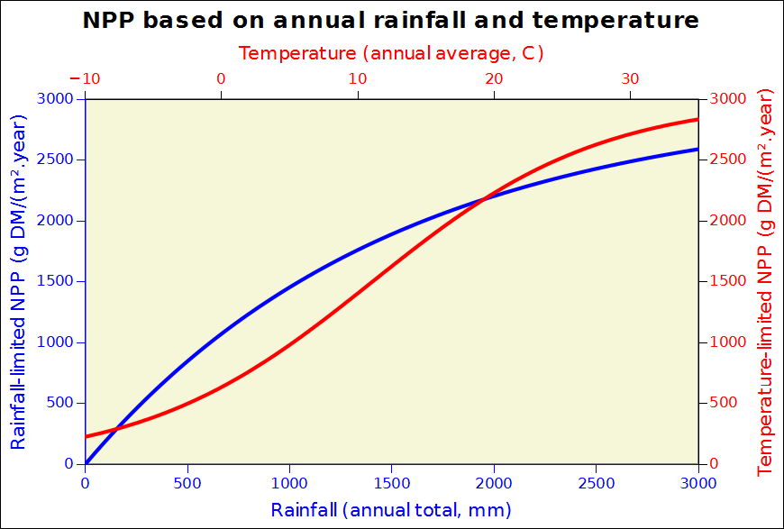
Figure 1: the variation of temperature and rainfall-limited NPP accrding to the Miami model with annual input data.

Both curves will eventually reach a (conventional) value of 3000 gDM/(m^2.day); they express the maximum production that can be achieved a a function of temperature (basically a proxy for solar energy) and water availability, two dominant limiting factors. For a given location, the minimum value of rainfall-imited and temperature-limited biomass accumulation is taken as the actual local production potential. Note that this is supposed to represent maximum annual biomass accumulation, which is different from standing biomass for perennials, including crops. The values expressed in gDM/(m^2.day) can easily be converted to tons biomass DM per Hectare: 1000 gDM/(m^2.day) is equivalent to 10 tons DM/Ha over one year, which would be about 3 tons of grain/Ha, considering that biomass is approximately partitioned into 50% of roots and 50% of above-ground biomass, of which, again, 50% can be assumed to be grain. This would be 2.5 tonnes DM. Making provision for some residual moisture, a value of 3 tonnes/Ha is probably an acceptable order of magnitude.Needless to say, actual values would depend on several additional factors, both crop specific and conditioned by the environmental conditions of growth such as water stress. Additional information can be found in Gommes et al 1999, 2009, 2010 as well as from the provided link. Global maps of Miami NPP are also available in GIS format from FAO or from here.

It is stressed that, while simple equations have gradually been superseded by satellite indices and model-based calculations, there is relatively little fundamental difference between the Miami model and and other well known and reputable approaches such as the CASA model of Potter et al (2007): both are empirically calibrated. There is more: both are basically potential production methods meant for planning rather than real-time or near real-time monitoring. In other words, regardless of the considerable variability that affects calibration data, the models can be used short-term monitoring. It is also stressed that there are several other empirical equations basically similat to the Miami “model”. Some are based on ETP, others on the length of growing season, on radiation etc. Some equations are very meaningful, for instance when they combine radiation (as source of energy to evaporate water) and water supply, as in the “Chikugo model”, but all have there shortcomings too. For instance, the Miami model pays no attention to the actual length of the growing season, relying on the statistical observation that long seasons are associated with larger amounts of precipitation than short ones. On the other hand, the mentioned Chukigo model, while very attractive because it incoporates latent heat of vaporization, rainfall and radiation, is not applicable in areas where frost occurs as temperature is not considered limiting. Another famous equation by Monteith combining radiation with a a cascade of “efficiences” has remained popular in many circles. The fact that all those more or less empirical equations as still fourty years after their first publication is a clear indicators of their usefulness. Refer to Gommes (1999) for additional  examples and a short discussion of the empirical biomass indicators and their uses.

14 sample points to compare Miami NPP approaches in monitoring

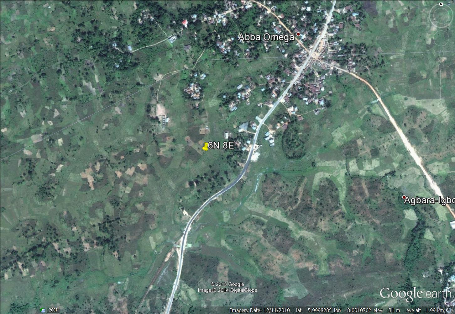
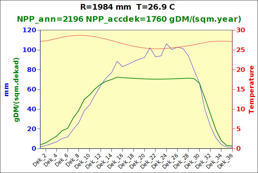
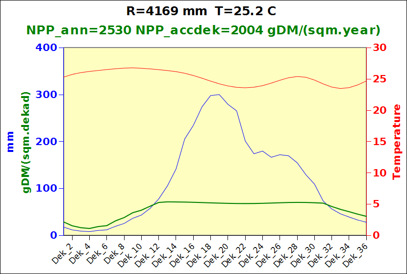
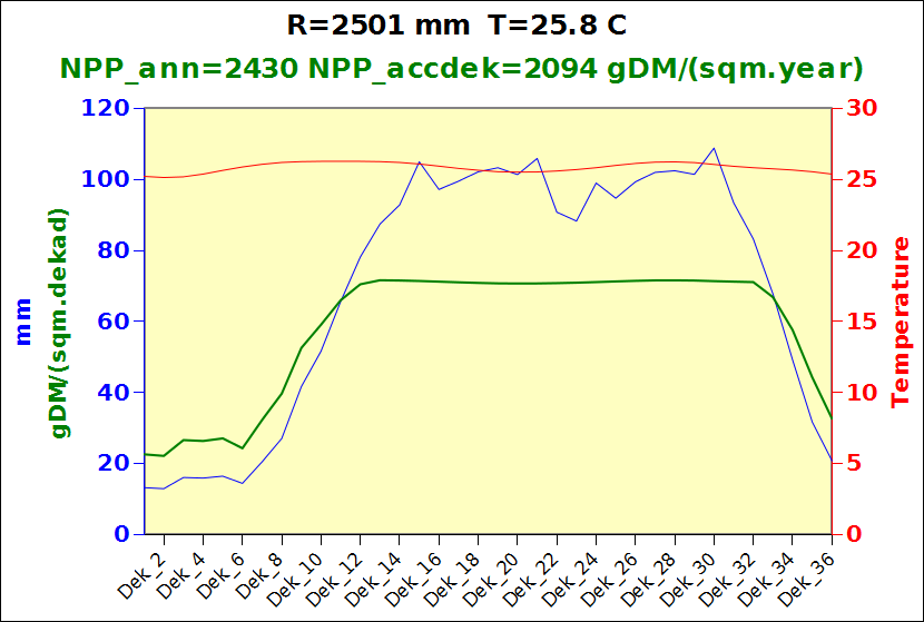
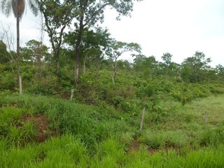
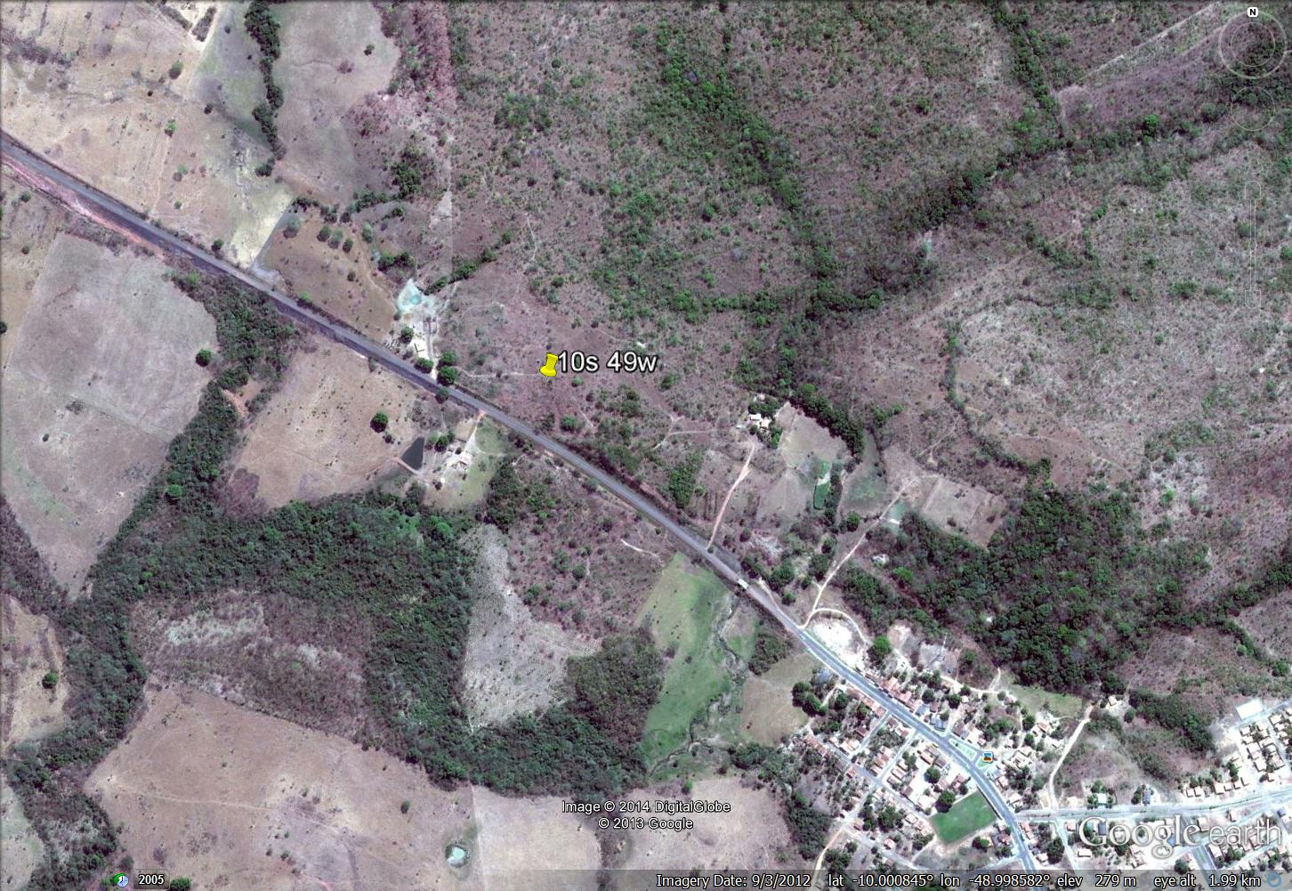
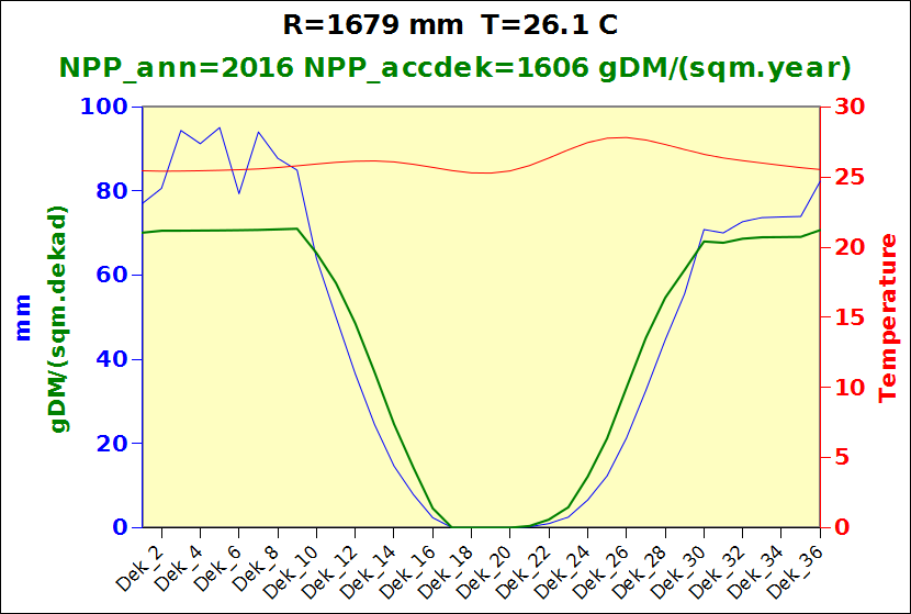
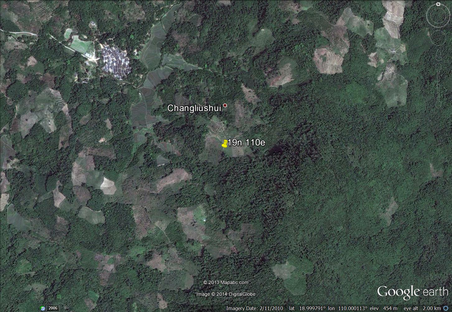
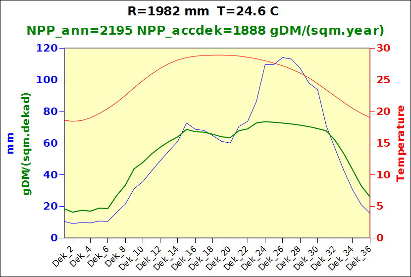
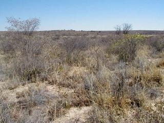
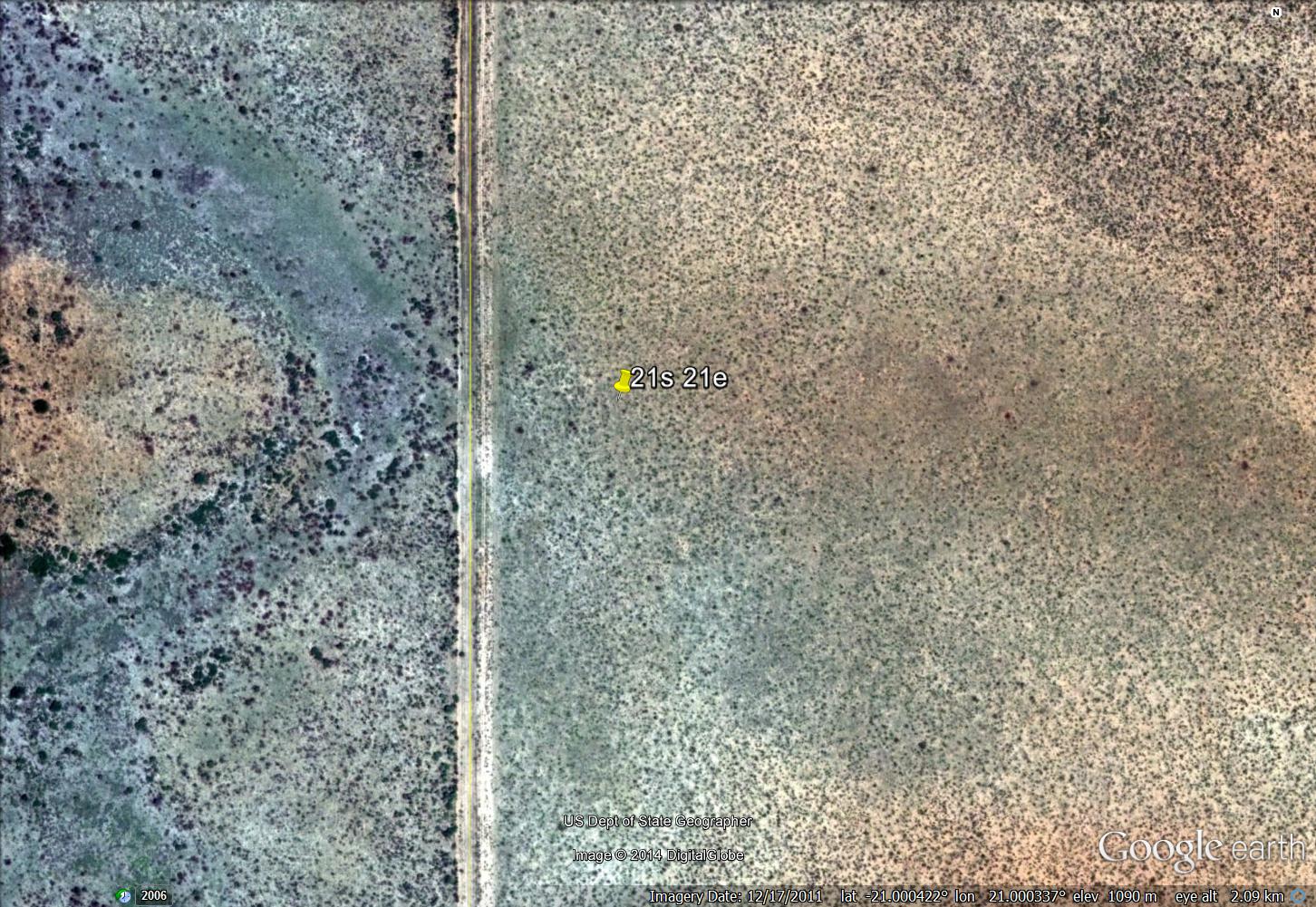
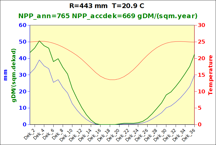
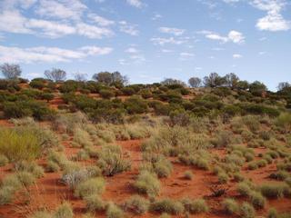
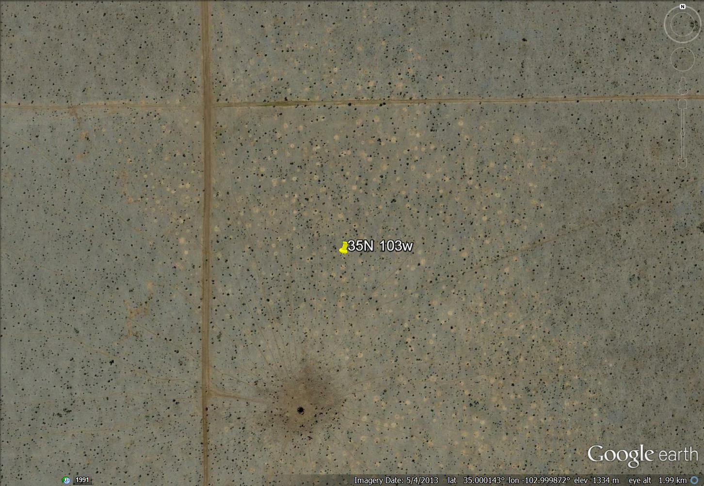
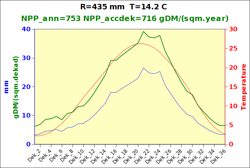
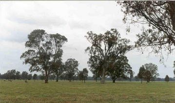
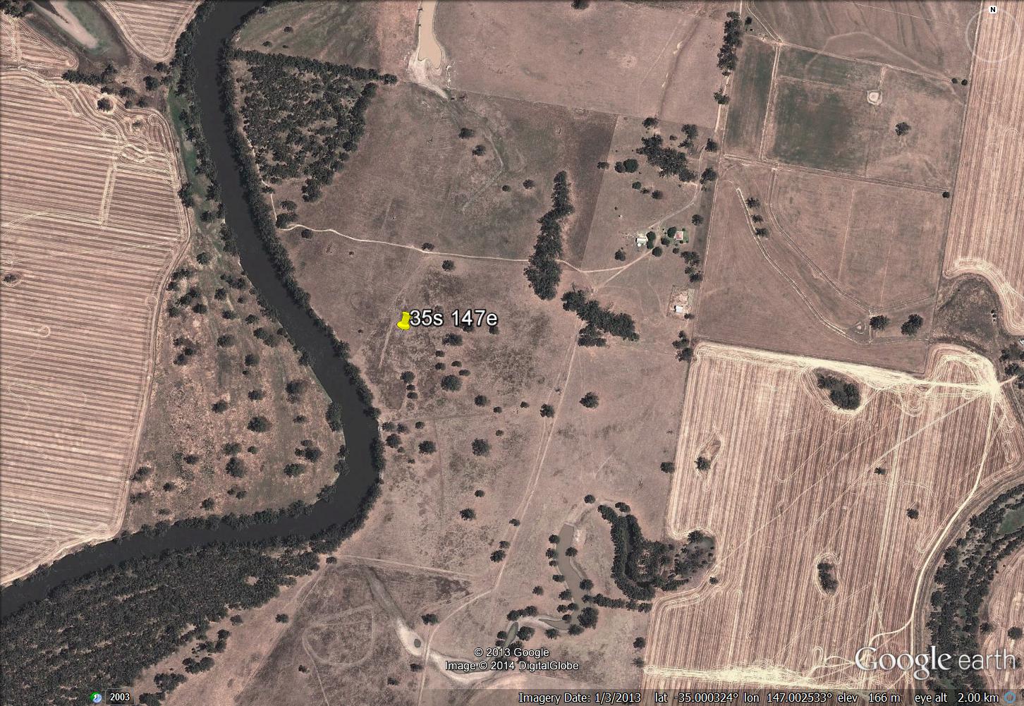
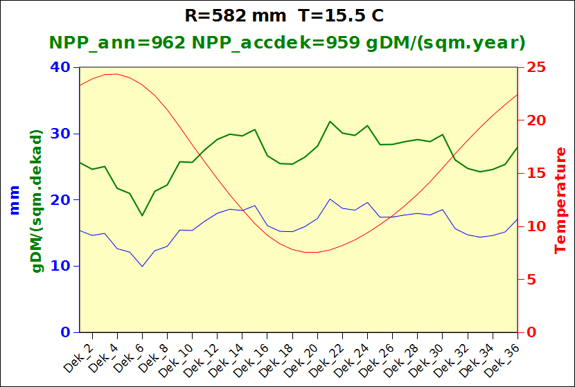
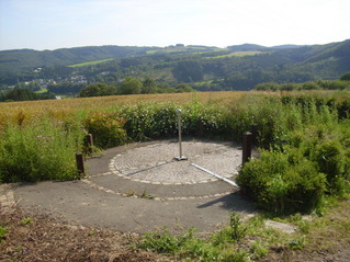
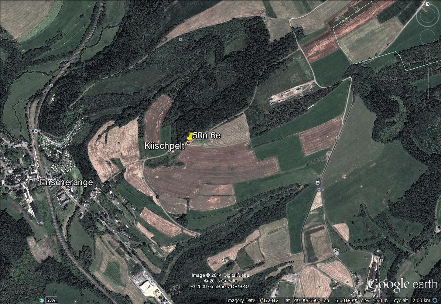
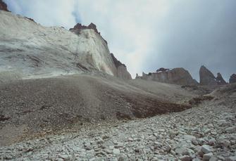
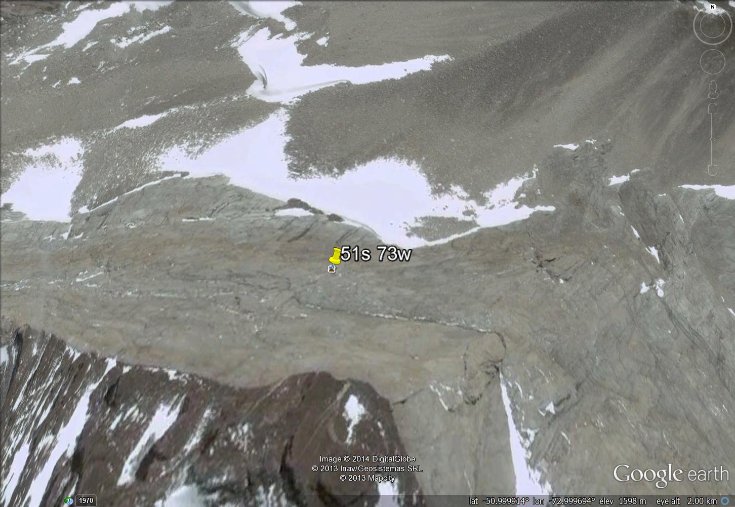
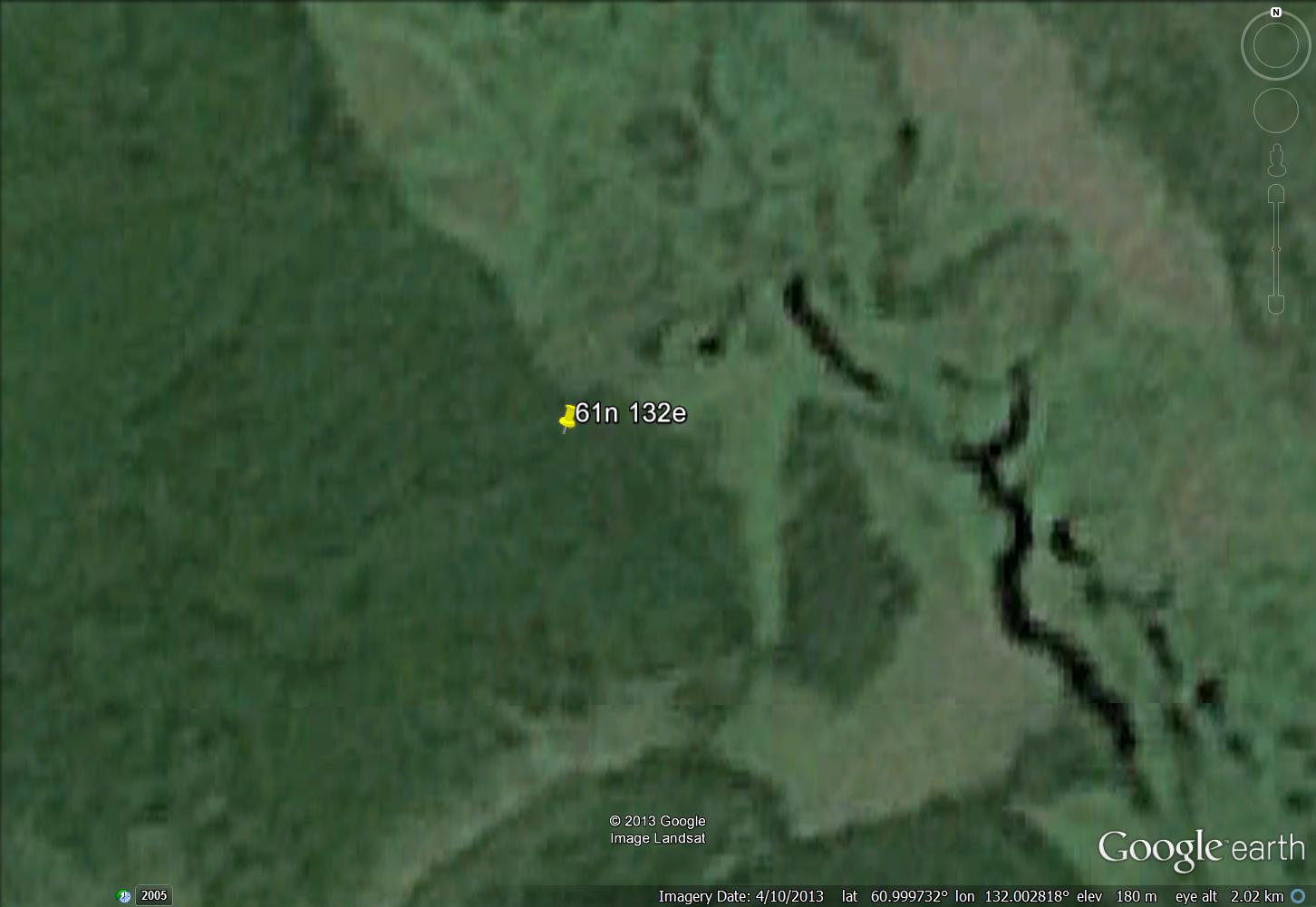
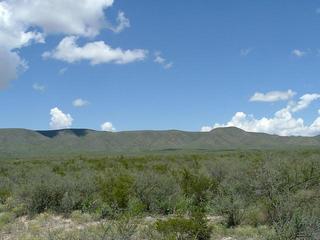
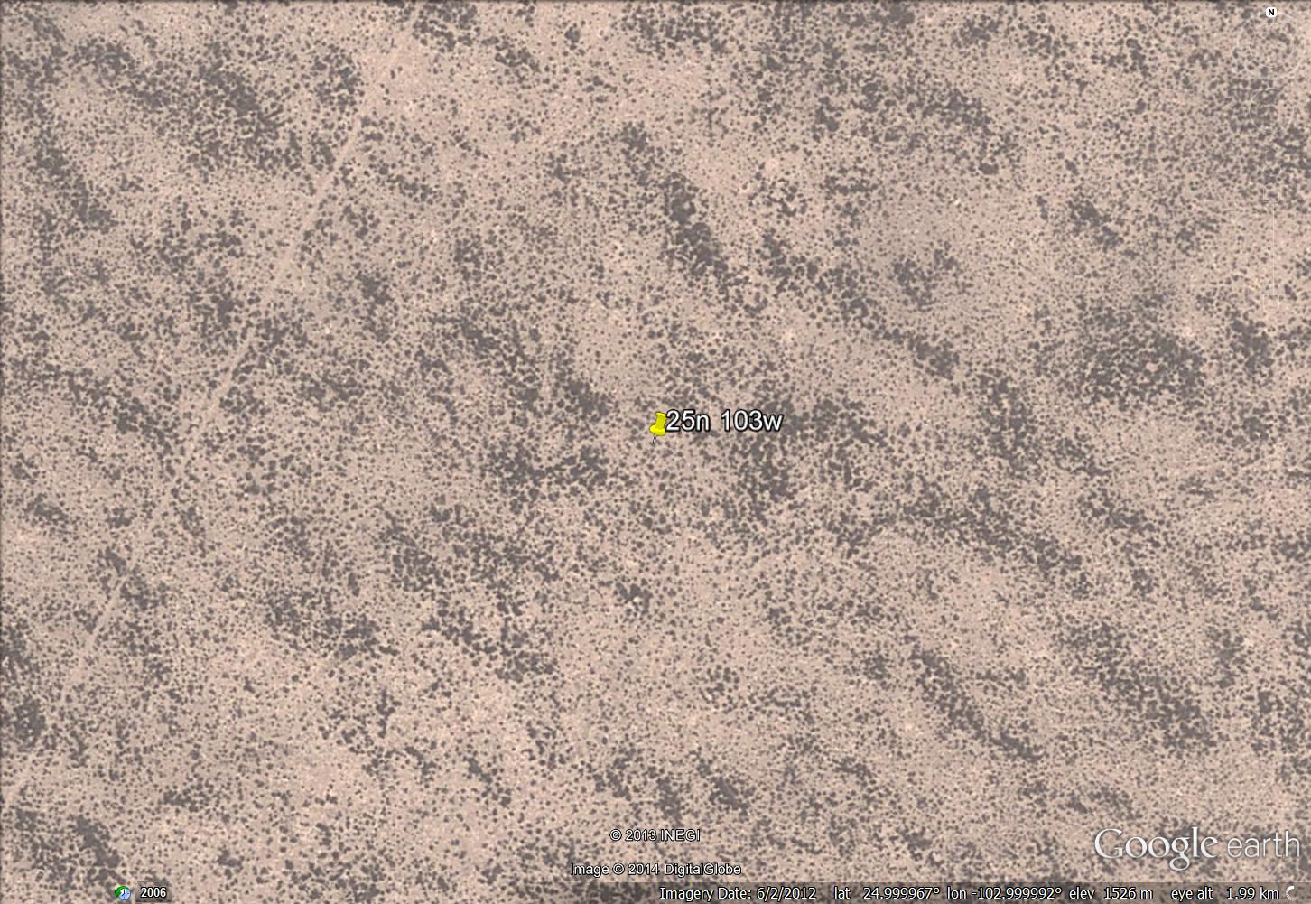
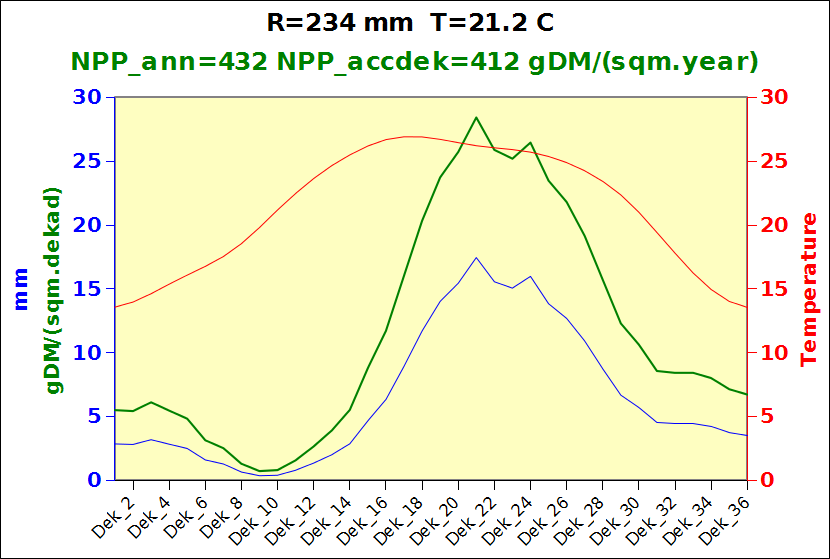
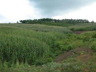
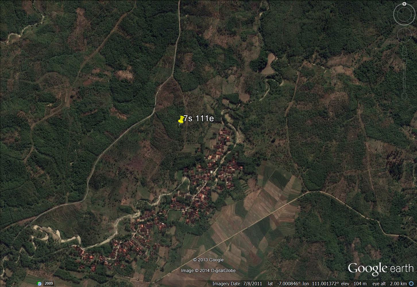
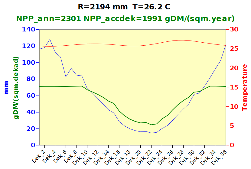
Before focusing on the different behaviours of “annual” and “dekad” Miami NPP, 14 points were selected across continents and climates to intuitively illustrate orders of magnitude of NPP and other indices in relation to climate and lanscape. They are shown in the table below, together with several classical climatic indicators:  the Köppen climate class, Budyko Radiation Dryness Index (RDI; dimensionless), Miami NPP (Net Primary Production potential in grammes of dry matter per square meter per year, gDM/(m^2.year)), Gorczynski continentality index (dimensionless), total annual rainfall (mm) and annual average temperature (deg. C) are all computed using the New_LocClim, software developed by Jürgen Grieser for FAO in collaboration with the German Weather Service, DWD. See this link to download the software and find out additional details about the listed indices. The pictures on the left were taken from the Degree Confluence project. The second “areal photograph” is a satellite image from GoogleEarth, corresponding to a view from an altitude of about 2000m. The views are clickable and provide also (Bottom right corner) the elevation of the area. The last column (climatic diagramme) was prepared with Gnumeric using data generated with New_LocCLim, i.e. resulting from a double interpolation: (1) spatially interpolated to the points of integer coordinates (2) dekad values estimated using Fourier interpoation from monthly averages.

Note that the value of “Miami NPP” corresponds to the value of NPP_1 described above. Also note that the values shown in the left column for NPP_1, Rain total (in mm) and Temp. average may slightly differ from those shown in the climatic diagramme of the last column due to rounding errors. The two NPP values given  under “Miami NPP dek.” are both dekad based and will receive additional attention below.The first corresponds to NPP_2 and the second to NPP_3.

008E 06N 100m asl near Afikpo, Nigeria
Köppen: BSh
Budyko RDI: 0.824
Aridity index: 1.26
Miami NPP: 2200
Continentality: 34.9
Miami NPP dek: 1760/1809
Rain total: 1984
Temp. avg.: 26.9
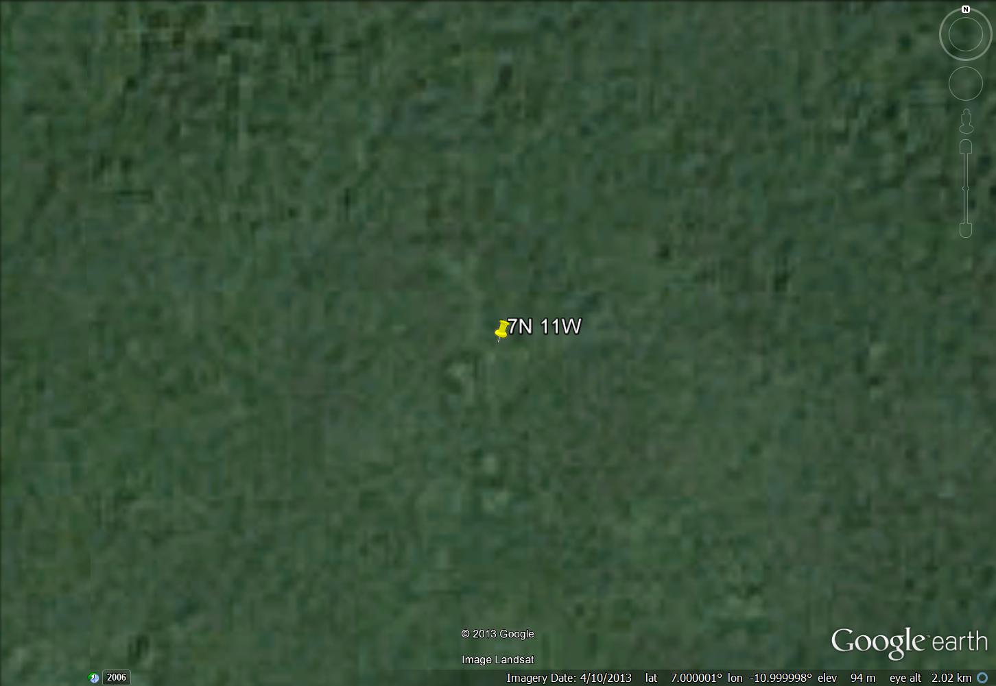
011W 07N 140m asl, south of Lofa Mano national park, Liberia
Köppen: BSh
Budyko RDI: 0.343
Aridity index: 3.26
Miami NPP: 2529
Continentality: 27.0
Miami NPP dek: 2004/2219
Rain total: 4169
Temp. avg.: 25.2
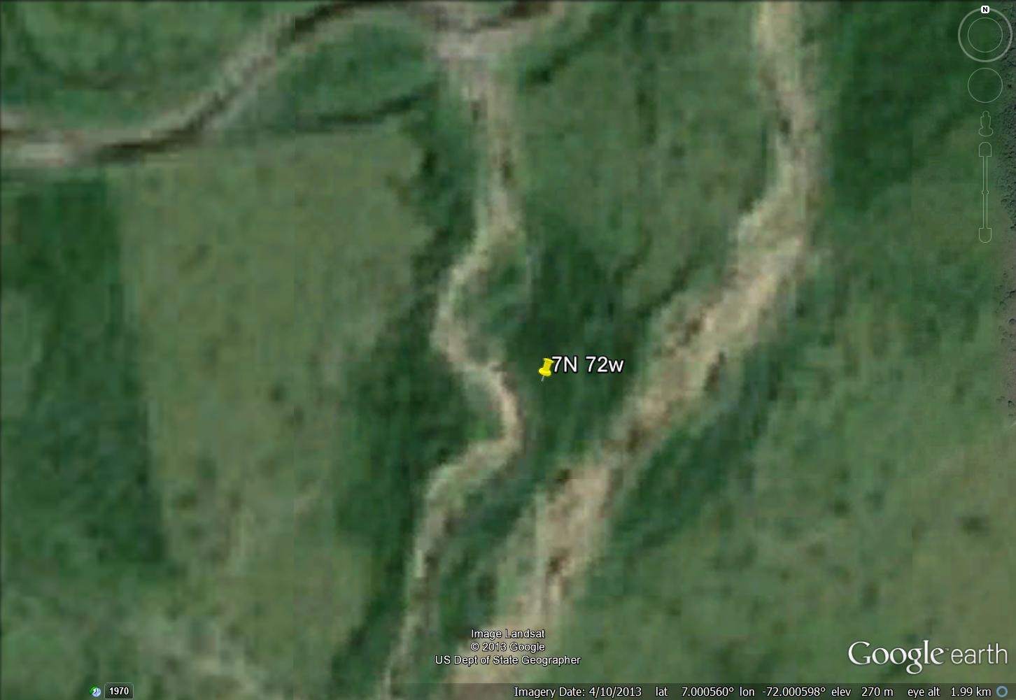
072W 07N 320 m asl, near Saravena, Colombia
Köppen: Aw
Budyko RDI: 0.716
Aridity index: 2.16
Miami NPP: 2432
Continentality: -3.7
Miami NPP dek: 2094/2174
Rain total: 2501
Temp. avg.: 25.8
111E 07S 200m asl,  near Purwodadi Java, Indonesia
Köppen: BSh
Budyko RDI: 0.884
Aridity index: 1.47
Miami NPP: 2298
Continentality: -0.9
Miami NPP dek: 1991/2047
Rain total: 2194
Temp. avg.: 26.2
049W 10S, 300m asl,  SE of Petrolina, Brazil
Köppen: BSh
Budyko RDI: 1.076
Aridity index: 1.17
Miami NPP: 2009
Continentality: 6.0
Miami NPP dek: 1606/1626
Rain total: 1679
Temp. avg.: 26.1
110E 19N 260m asl, Hainan Island, China
Köppen: Aw
Budyko RDI: 0.817
Aridity index: 1.58
Miami NPP: 2198
Continentality: 33.9
Miami NPP dek: 1888/1922
Rain total: 1982
Temp. avg.: 24.6
021E 21S 1060 m asl, NE Namibia
Köppen: BSh
Budyko RDI: 3.641
Aridity index: 0.3
Miami NPP: 758
Continentality: 31.8
Miami NPP dek: 669/669
Rain total: 443
Temp. avg.: 20.9
127E 25S 460 m asl, Central western Australia
Köppen: BSh
Budyko RDI: 8.464
Aridity index: 0.07
Miami NPP: 336
Continentality: 53.6
Miami NPP dek: 335/335
Rain total: 179
Temp. avg.: 22.4
103W 35N 1240 m asl, between Tucumcari (New Mexico) and Amarillo (Texas), USA
Köppen: BSk
Budyko RDI: 3.051
Aridity index: 0.24
Miami NPP: 754
Continentality: 49.8
Miami NPP dek: 716/716
Rain total: 435
Temp. avg.: 14.2
147E 35S 140 m asl, NE of Wagga Wagga, New South Wales, Australia
Köppen: Cfa
Budyko RDI: 2.336
Aridity index: 0.44
Miami NPP: 964
Continentality: 27.9
Miami NPP dek: 959/959
Rain total: 582
Temp. avg.: 15.5
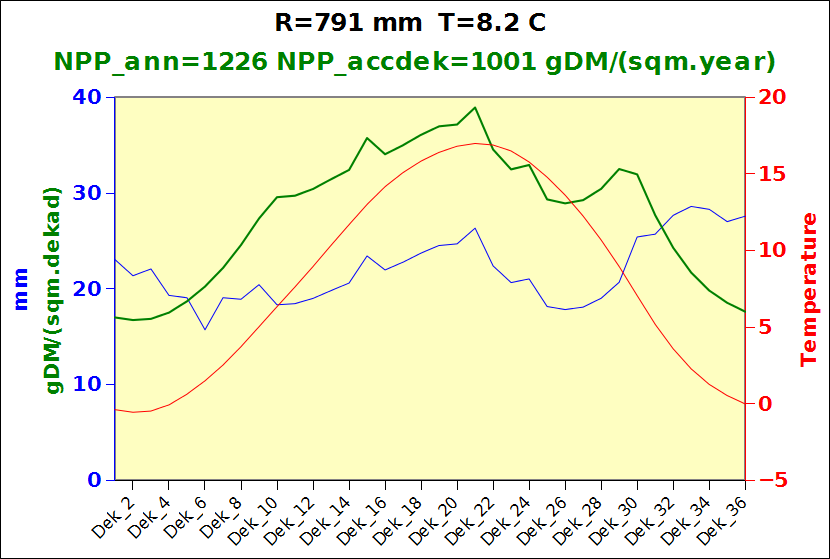
006E 50N 440 m asl, near Kiischpelt, Luxembourg
Köppen: Cfb
Budyko RDI: 1.055
Aridity index: 1.33
Miami NPP: 1227
Continentality: 17.8
Miami NPP dek: 1001/1220
Rain total: 791
Temp. avg.: 8.2
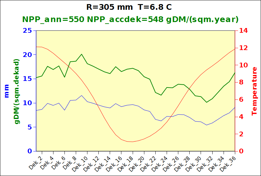
073W 51S 1160 m asl, Torres de Paine National Park, Chile
Köppen: Cfc
Budyko RDI: 2.392
Aridity index: 0.45
Miami NPP: 548
Continentality: 3.2
Miami NPP dek: 548/548
Rain total: 305
Temp. avg.: 6.8
132E 61N 220 m asl, Eastern Siberia, Russia
Köppen: Dfd
Budyko RDI: 1.183
Aridity index: 0.79
Miami NPP: 230
Continentality: 94.7
Miami NPP dek: 412/539
Rain total: 310
Temp. avg.: -9.9
103W 25N, 1500m asl, near Monterrey, Mexico
Köppen: Bwh
Budyko RDI: 5.302
Aridity index: 0.20
Miami NPP: 433
Continentality: 33.5
Miami NPP dek: 412/412
Rain total: 234
Temp. avg.: 21.2

Computation of Miami NPP with annual Vs dekadal data

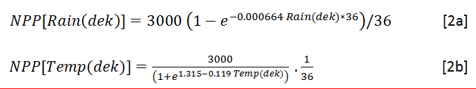
Two approaches (NPP_2 and NPP_3) were explored to compute Miami NPP based on dekadal data. Both start with the calculation of “dekadal NPP”, which can be interpreted – ideally – as the contribution of each dekad to the annual NPP. NPP_2 and NPP_3 are both based on dekad climate variables for dekads dek=1 to 36 (one complete season, or sometimes a shorter period), Rain(dek) and Temp(dek). First compute the contribution of each dekad to annual NPP

The equations below explain the difference between NPP_2 and NPP_3.

In the case of NPP_2, for each dekad compute

and then sum dekad values

For NPP_3, sum all values for rainfall-limited dekad NPP NPP[Rain(dek)] and temperature-limited NPP NPP[Rain(Temp)]

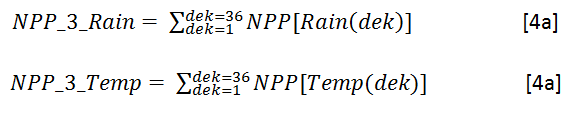and take the minimum of the two sums

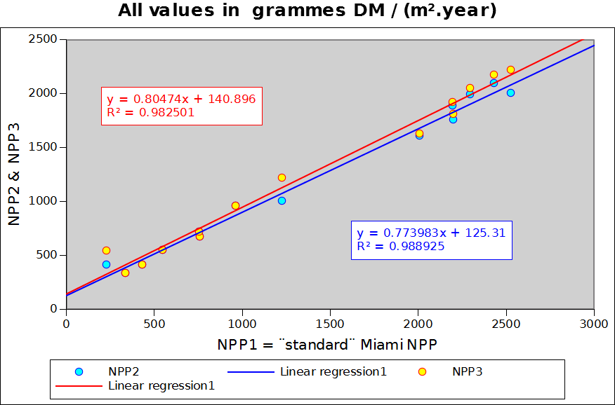
Figure 2: dekad-based Miami NPP Vs annual-based.

Figure 2 compares NPP_1, NPP_2 (in blue)  and NPP_3 (in red)  for the 14 sample points of the previous section. Correlations appear to rather good but the regression coefficients do markedly differ from 1 (0.805 for NPP_3 and 0.774 for NPP_2). In other words both NPP_2 and NPP_3 understimate NPP over the annual vegetation and climate cycle. This is, however, a minor issue in monitoring terms, as we are not considering NPP in absolute terms but as an indicator capable of integrating both rainfall and temperature. The absolute value of the indicator is of little relevance.

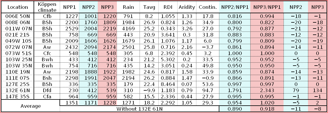
The table below shows NPP_2 and NPP_3 as well as other indices for the 14 locations. It provides some additional information about the order of magnitude of the difference between NPP_1, NPP_2 nd NPP_3 over a wide spectrum of environmental conditions. NPP_2 and NPP_3 systematically underestimate NPP_1 by about 0 to 20% (the two last columns express the % error which results from using NPP_2 or NPP_3 instead of NPP_1. One point differs markedly from all the others: 132E 61N (Eastern Siberia) in a location where birch and lark apparently make up the sparse woody vegetation. The point provides a good illustration of the need to consider both standing biomass and NPP.  The area is characterised by a very cold climate (Dfd) with an average annual temperature close to -10 degrees. Obviously a very fragile ecosystem where biomass replacement (and decay) occur very slowly. It is obvious that, in this case, the dekadal temperature curve is too optimistic, as no growth is certainly to be expected at below zero temperature.

Comparison of NPP_1, NPP_2 and NPP_3 using randomly simulated data

It appears that some additional exploration of the relative behaviour of NPP_1, NPP_2 and NPP_3 is required, to better understand the role of rainfall and temperature, in particular the differences to be expected as a function of the relative timing of high temperatures (i.e. growth compatible temperatures) and the rainy season. Obviousy, a lot of empirical knowledge went into the standad Miami NPP equations (NPP_1). For instance, it could be assumed that whenever precipitation coincides with the cold season (mostly as snow), with no additional rain falling during the warmer season, the outcome should be no production potential and no vegetation. This is not so, however… at least not statistically: moisture is stored above the ground as snow and below the ground in the root zone, and becomes available during the time of snow melt, even if the growing period is very short. This explains why the curves selected by Lieth differ markedly at low values, in order to account for non-zero NPP at negative temperatures. This makes perfect sense with annual data, but becomes meaningless when considering dekadal NPP. The observation also explains why, as will be shown below, NPP_3 provides more meaningful and consistent data than NPP_2: the summation somehow restores the statistical validity that is inherent in NPP_1.

A simple model was built using the Gnumeric spreadsheet to test the effect of the relative timing of rainfall and the warm season on the validity of NPP_2 and NPP_3 as biomass monitoring tools. The figure below shows two different and contrasting simulation runs.

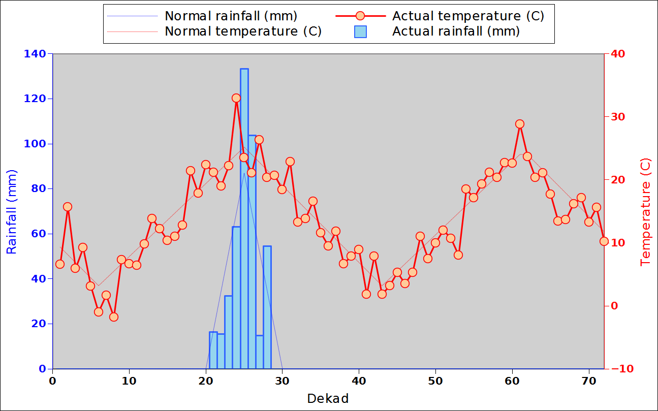Figure 3 (A): a sample run of the spreadsheet showing simulated dekad temperature and dekad rainfall to be used to compute dekad-based and annual-based Miami NPP.

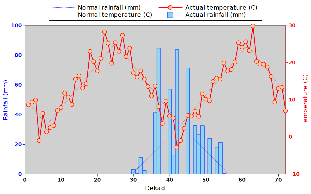Figure 3 (B): another sample run of the spreadsheet showing simulated dekad temperature and dekad rainfall to be used to compute dekad-based and annual-based Miami NPP.

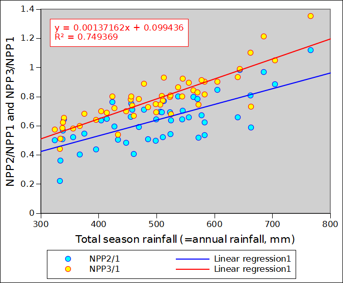Figure 4 (A): Ratio of NPP_2/NPP_1 and NPP3/NPP_1 as a function of total seasonal rainfall.	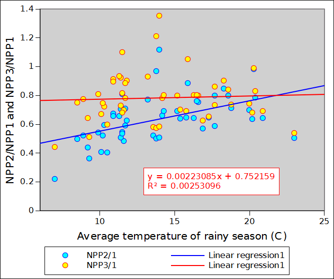Figure 4 (B): Ratio of NPP_2/NPP_1 and NPP3/NPP_1 as a function of the average temperature of the rainy season, i.e. the temperature of the period during which precipitation is available.	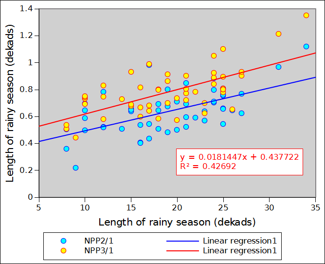Figure 4 (C): Ratio of NPP_2/NPP_1 and NPP3/NPP_1 as a function of the length of the rainy season in dekads.
(A)	(B)	(C)

Conclusion

Miami NPP can be computed based on dekad values of rainfall and temperature. Correlations between the standard Miami NPP based on annual rainfall and temperature and two variants of dekad-based calculations are very high, confirming that, statistically, the dekads values can be used since NPP is used as an indicator: spatial variations and inter-annual variations are preserved. In general, dekad-based NPP underestimates NPP by about 20%, except in very cold locations where crop agriculture is unlikely to be practiced. For a given location, the ratio between dekad-based NPP and annual-data-based NPP varies as a function of rainfall: high ratios are associated with high temperature values. Finally, the variant of dekad-based NPP described as NPP_3 is generally a better choice that variant NPP_2. It is, therefore, recommended for crop monitoring with the Miami equations when dekad data are used.

References

Bouman BAM, Van Keulen H, van Laar HH, Rabbinge R, Van Keulen H 1996 The ‘School of de Wit’ crop growth simulation models: a pedigree and historical overview. Agricultural-Systems, 52(2-3):171-198.

de Wit CT, Goudriaan J, van Laar HH, Penning de Vries FWT, Rabbinge R, van Keulen H, Louwerse W, Sibma L, de Jonge C 1978 Simulation of assimilation, respiration and transpiration of crops. Pudoc, Wageningen, 141 pp.

FAO 1978–81 Report on the Agro-ecological Zones Project. Vol. 1. Methodology and results for Africa. World Soil Resources Report 48/1, FAO, Rome.

FAO 1980 Land Resources for Populations of the Future. Report of the Second FAO/UNFPA Expert Consultation. FAO, Rome.

Gommes, R. 1999. Roving Seminar on crop-yield weather modelling; lecture notes and exercises. WMO. Geneva, 153 pp. ftp://ext-ftp.fao.org/SD/Reserved/Agromet/Documents/agro003a.pdf.

Gommes R, Das H, Mariani L, Challinor A, Tychon B, Balaghi R, Dawod MAA 2010 Agrometeorological Forecasting. Chapter 6 of WMO Guide to Agrometeorological Practices (GAMP), WMO N. 134 Geneva 49 pp, http://www.wamis.org/agm/gamp/GAMP_Chap06.pdf

Gommes R, El Hairech T, Rosillon D, Balaghi R, Kanamaru H 2009 Impact of Climate Change on agricultural yields in Morocco. World Bank-Morocco study on the impact of climate change on the agricultural sector. 105 pp. Downloadable from ftp://ext-ftp.fao.org/SD/Reserved/Agromet/WB_FAO_morocco_CC_yield_impact/report/

Lieth H 1972 Modelling the primary productivity of the world. Nature and Resources, UNESCO VIII 2:5-10.

Lieth H 1973 Primary production: Terrestrial ecosystems. Human Ecology 1(4)303-332.

Meadows DH, Meadows G, Randers J, Behrens WW 1972 The Limits to Growth. New York: Universe Books

Potter C, Klooster S, Huete A, Genovese V 2007 Terrestrial Carbon Sinks for the United States Predicted from MODIS Satellite Data and Ecosystem Modeling, Earth Interactions 11(13) 21 pp.

Annex: spreadsheet simulation to compare annual (NPP_1) and dekad-based (NPP_2 and NPP_3) NPP using the Miami model

The calculations were carried out with the Gnumeric spreadsheet (*) downloadable below. The spreadsheet also contains two sheets explaining how to compute series of statistical data following the Weibull and the normal distribution. The original intention was to use the Weibull distribution for both rainfall and temperature, as this would have allowed to simulate the positive skew affecting rainfall (especially low values) as well as the the positive skew that is often observed with temperatures. Eventually, to simplify and accelerate things, a normal distribution was adopted; it is suggested that the simulation would only have been marginally improved using the Weibul distribution.

The sample outputs illustrated in figure 3(A) and (B) correpond to the same input values. The figures are based on a number of random numbers used to simulate climate data. The random numbers where reactivated between the two runs. A rotal of 50 runs was carried out, as a larger number would require a different tool.

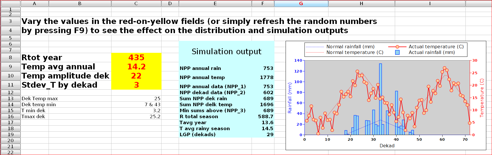
Figure 5: the spreadsheet used to compute the figures 3 (A) and (B) and to estimate the values of NPP_1, NPP_2 and NPP_3 nd other variables that are used in figure 4.

A note follows about the derivation of the equation that was used to estimate standard deviation of rainfall as a function of total rainfall. Figure 6 was prepared based a dekadal Ethiopian data between 1991 and 2009 in 9 stations. The fact that Etiopia was selected is irrelevant, as the intention was just to derive a typical relation between average rainfall and standard deviation at the dekadal scale. The relation was subsequently fitted with CurveExpert which indicated that the Vapour pressure equation was the second best.

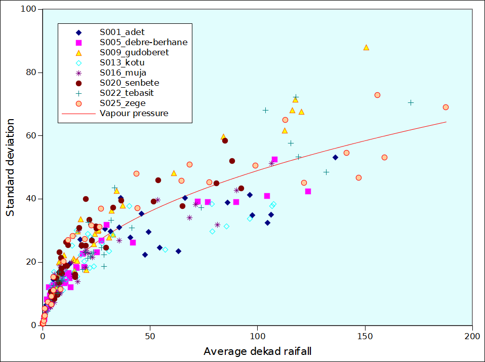
Figure 6: Standard deviation of dekad rainfall for 36 dekads in 9 Ethiopian stations between 1991 and 2009 (19 years). The red line corresponds to the Vapour Pressure equation fitted through the 252 data points.

(*) See the provided links to download Gnumeric for Linux or for Windows. No apologies are offered for using the best spreadsheet currently available for scientific work. The spreadsheet was saved using different Excel and open document formats; the gnumeric version is the original; some formatting was probably lost in the other formats.

Download spreadsheet as Gnumeric: gnumeric , odf_1: Miami-npp-dekad-vs-annual-inputs_1, odf_2: Miami-npp-dekad-vs-annual-inputs_2, excel_1: Miami-npp-dekad-vs-annual-inputs_1, excel_2 Miami-npp-dekad-vs-annual-inputs_2, excel_3 Miami-npp-dekad-vs-annual-inputs_3