Experts I’ve interviewed over the past six years generally agree that such a Next
Big One is not only possible but probable. They agree that it will almost certainly be a zoonotic disease — one that emerges from
wildlife — and that the causal agent will most likely be a virus. They agree that sheer human abundance, density, and
interconnectedness make us highly vulnerable.
David Quammen, The Next Pandemic: Why
It Will Come from Wildlife
First published 20110929 – Last updated on 20121009
1. Introduction
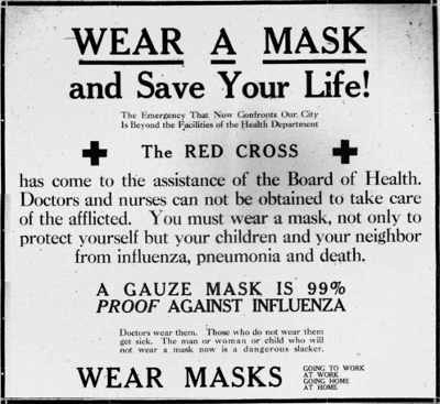
This public notice (taken from an article by J. Barry, 2009) was used in San Francisco in 1919 to warn people against the Spanish flu. Barry’s legend mentions that bold declarations like this one from San Francisco were rare in 1918.
In March and early April 2009, a new swine-origin influenza A (H1N1) virus (S-OIV) emerged in Mexico and the United States. During the first few weeks of surveillance, the virus spread worldwide to 30 countries (as of May) by human-to-human transmission, causing the World Health Organization to raise its pandemic alert to level 5 of 6. This virus has the potential to develop into the first influenza pandemic of the twenty-first century (Smith et al, 2009).
In early-November 2009, we heard that the influenza A peak has been reached; a couple of days later, the news reported on 20091120 that a Norwegian patient had died from a mutated H1N1, after which the French, followed by several others too found a mutated virus; on 20091129, we were told that the mutation spreads and that India waits for the vaccine. Should we worry more than we did? Possibly, or maybe not, because as early as 7 days ago (20091122), experts had told us that the vaccines are effective against the mutated virus. At this stage I wonder if there is anyone around who does know! Health authorities wave the precautionnary principle flag (remember the 2003 heatwave?) , and the business of tamiflu makers is as good as ever! Maybe our fears are like high food prices, i.e. they are driven by demand, and by offer as well!
I decided to publish this post because, a couple of years back (20051113), I had written a little “model” and a note for myself after reading the well-known book by Malcolm Gladwell on The tipping point, how little things can make a big difference. The book is about the many socio-economic variables around us that, for no immediately obvious reason, suddenly undergo rapid growth or decline. This includes fashions, book sales (what makes a best-seller?), crime rates in large cities, teenager smoking and many others, including epidemics.
The book has an end-note explaining how density of population plays a critical role in the spreading of epidemics. Below a threshold value, the epidemic dies out, while it expands rapidly at higher densities. Gladwell provides a hypothetical example of a group of tourists visting Manhattan. It is assumed that the tourists are infected with “24 hours flu” and that they use the subway a lot. If they visit during summer, when the subway is not very crowded, nothing happens. If, on the other hand, they visit before christmas when the subway is crowded, there is the potential for starting an epidemic. There is a specific “tipping point” value of the number the tourist come in contact with below which there will be no epidemic. Above the tipping point, an epidemic will be started.
What is, maybe, more interesting, is that systems with tipping points may exhibit some characteristics that could be used to warn of an imminent change of regime. This is the subject of a recent review article by Scheffer et al. (2009) in Nature. To quote from the article, complex dynamical systems, ranging from ecosystems to financial markets and the climate, can have tipping points at which a sudden shift to a contrasting dynamical regime may occur. Although predicting such critical points before they are reached is extremely difficult, work in different scientific fields is now suggesting the existence of generic early-warning signals that may indicate for a wide class of systems if a critical threshold is approaching. One of the symptons Scheffer lists is critical slowing downof variability before a “catastrophe” is reached (the system “hesitates”). Incidentally: the authors never refer to René Thom, the inventor of catastrophe theory, while they use his terminology a lot!
2. The N-flu tipping point model
I call the little model I mentioned above the N-flu tipping point model; it can be used to simulate the tipping point behaviour in the case of epidemics. Why N-flu? Because an individual is assumed to be ill and contagious for N days. The model is very simple, and it probably has no relevance to the reality of the complex pandemic risk we seem to be exposed to (Yang Yang et al., 2009). But it does illustrate that, even with very simple assumptions, the tipping point mechanism can be shown very easily, as in the figures below.
Anyone interested can have a look at section 3, where a full description of the N-flu model is provided, as well as the spreadsheet that implements it.
The N-flu model is controlled by three variables and by the initial fraction of the population that has already caught the virus. The fraction is F, i.e. if F=0.5, every second persons carries the virus.
The variables are:
- N, the number of days a person remains sick and during which it can contaminate others;
- n, the population density; note that the density is an arbitrary number; it is not the real population density in persons/(km.km). Density is an all important variable, as I have stressed some time ago with three colleagues in the case of HIV/AIDS (Gommes et al., 2004);
- P, the infectivity, i.e. the proportion of persons exposed to the N-flu virus who become infected by it. In other words: if I carry the N-flu virus, and P=0.2, two out of 10 people I meet will catch the virus from me.
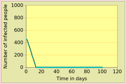
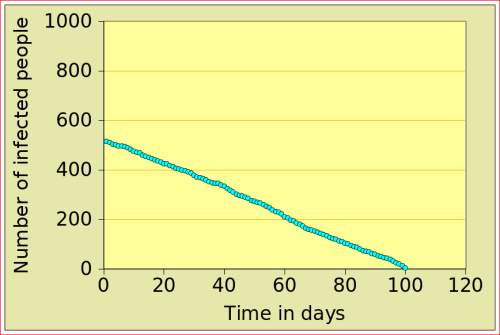
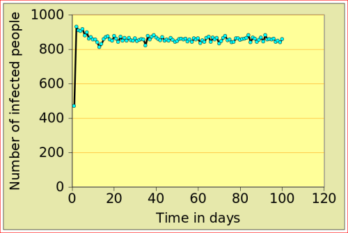
For now, just look at the figures below: they show the number of people affected by N-flu (out of a total population of 1000) , as a function of two variables: the period N(days) over which a infected person remains contagious, and population density (n). Start with the graphs in the top row. On the left, N=12 and n=10: after just over 10 days, the epidemic dies out, from 500 people affected to 0. On the right, the flu is assumed to make people contagious for 100 days, with a very low population density of 2. The epidemic very slowly does out.
Now look at the bottom left figure: the variables are the same as in the top left figure, with the exception of the density, which increases from 10 to 11: that simple increase of 1 leads to a completely different behaviour of the epidemic: the number of people affected jumps to above 800, and stays there. There is a tipping point between 10 and 11 (more precisely between 10.729 and 10.730!)
|
N-Flu type: N=12; population |
N-Flu type: N=100; population |
|
N-Flu type: N=12; population |
The values of F and P below were used for all the simulations shown. F=0.5, initial value of fraction of population infected P=0.2, probability of catching N-flu when meeting an infected person. |
A runaway situation occurs when one of the model variables passes the threshold, the other variables being “fixed”, as in the example above: the epidemic starts when densiry n changes from n=10 to n=11, provided that we have N= 12 (12-day flu), F=0.5 (initial value of fraction of population infected) and the probability of catching N-flu when meeting an infected person is P=0.2 (2 chances in ten). If I change the value of P (i.e. if the virus mutates and becomes more contagious), then there will also be a different value of density n associated with it. By using the N-flu model spreadsheet given below in section 3, it is possible to systematically vary P from 0.001 to 1 and then determine the associated density value n. This is shown in the graph below (left) where, in addition, the the value of F has also been changed from N-0.1 to N=0.3 and N=0.5.
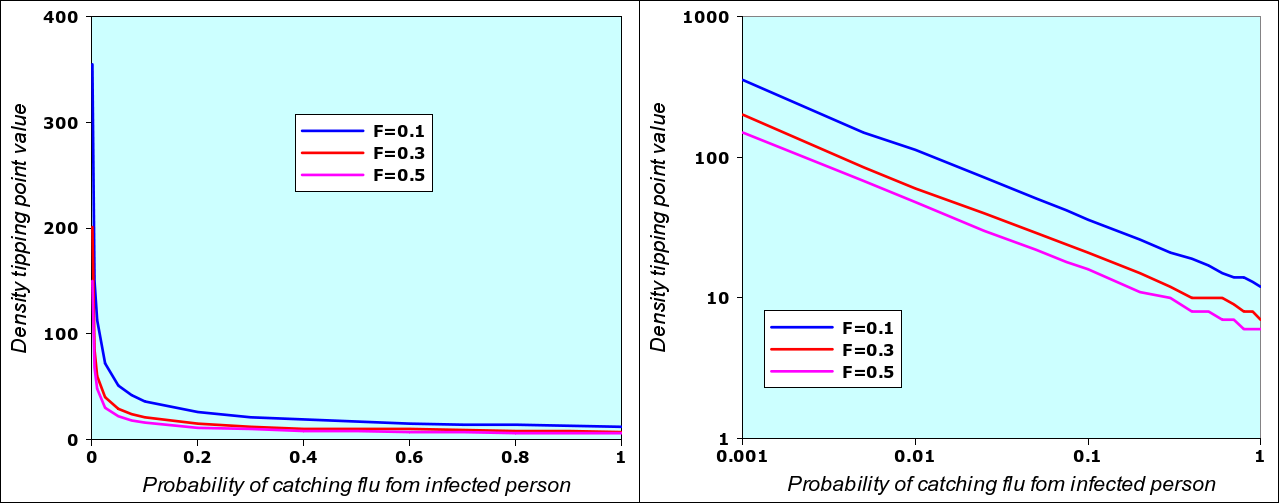
Value of density that triggers an epidemic for different values of “infectivity” P and three different values of F (initial fraction of population being infected). The two graphs are identical: the left one adopts a linear scale, the one on the right has an logarithmic scale. The reason why the logarithmic scale works has to do with the way the “number of people met per day” (one of the internal moel variables) varies as a function of density. The detailed description of the model will give interested readers an explanation why this is so. I repeat that I don’t know if this corresponds to the real reality of epidemics.
What this also means is that, in real situations, any variables can be a trigger: you can “fix” the value of density, and vary the infectivity. Logically, if infectivity increases, then the density required to start the epidemic is lower. Within the range of acceptable values (and within the limits of the N-flu model), for every value of P, we have a trigger value of n, and for every n, we have a corresponding trigger value of P. Since the n-P graph can easily be linearized, we can also easily compute one of the trigger values when the other is known, as in the equations below for F=0.5.
The graph below is the same as the rightmost graph in the figure above (the purple curve only, i.e. F=0.5).
Under the purple line (described by the equations above), the values of n and P are such that no epidemic occurs. Assume n=10: in this case, the epidemic
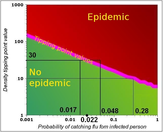
Some examples of n-P couples that can trigger an epidemic with F=0.5. Both above and below the tipping point line, the system is “stable”. All the n-P couples above the line that correspond to an epidemic. For all n-P couples below the line, the virus dies out in the population. Strictly, only the tipping point (purple line) is unstable, as a small departure from the line leads the system either into an epidemic or into the gradual reduction of the number of people affected.
will start if P>0.28. This can also be expressed as follows: if the infectivity is P=0.28, then the trigger occurs at n=10.
Now assume n=30 and P=0.017. WE are in tge “stable region” as we are below the tipping point value of P=0.022. IF the virus mutates, and the infectivity increases to 0.048, the epidemic will start.
In reality, we live in a situation where all the variables keep fluctuating over time and space, with islands where tipping points are being reached, and others where the problems subside.
We can imagine that islands grow and shrink and sometimes coalesce; when they do, there is potential for a larger explosion and a pandemic…
At this stage, I would like to come back to the more fundamental issue of tipping points in general, that occur in many circomstances, for instance in the area of desertication: the variables are climate and especially rainfall, cattle and people density (as vegetation is used for animal grazing, but also as firewood), type of soil (more or less sandy; more or less degraded), type of vegetation and type of animals, frequency of fires, etc. All the variables together define a system and the nature of the tipping points. If we define desert simplistically as the absence of vegetation, then pockets of desert appear in vegetated areas. They sometimes recover (e.g. seeds are flown in by wind, or maybe even planted by people), and they sometimes expand. When the pockets grow and merge, the risk is higher that seeds will no longer germinate or grow, for natural and man-made reasons. Eventually, if the pockets meet with the Sahara, we will say the the Sahara expands…
We can apply the same reasoning to biodiversity, and the “intermediate disturbance hypothesis”, which is very similar to the desertification mechanism just described: biomass and biodivesiy destruction can be taken up to a certain point only.
Tipping points are averywhere.
3. Technical details
Technical details can be obtained by downloading the description of the model, by clicking here. The Gnumeric spreadsheet (tar.gz, 656 KB) can be downloaded from here, while the Excell version is availble here (2.2 MB, zipped).
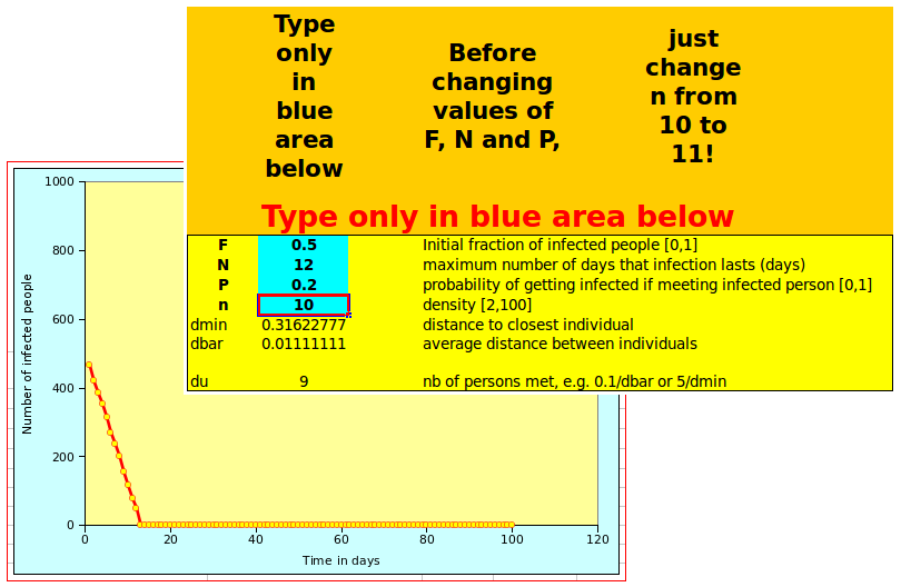
Both spreadsheet look the same and work the same way: on the left of the screen, there is a graph showing the number of affected people over time. On the right, the user can define the parameters in the box with a blue background, as shown below:
Changing n from 10 to 11 will display the tipping point behavious illustrated above. Once you have suceeded doing that, you can start playing with other parameters! Note that, depending on the settings of your spreadsheet, you may need to recalculate the values, as otherwise the graph will not be updated automatically.
4. References
John M. Barry, 2009. Pandemics: avoiding the mistakes of 1918. Nature, 459:324-325.
M. Gladwell, 2002. The tipping point, how little things can make a big difference. Black Bay Books (Paperback), 304 pp. The first (hardcover) editions was published in 2000.
R. Gommes, J. du Guerny, M.H. Glantz and Lee-Nah Hsu, 2004. Climate and HIV/AIDS: a hotspots analysis for early warning rapid response systems. UNDP/FAO/NCAR, UNDP SE Asia and Development Programme, Bangkok, 20 pp. Available from FAO or from here HIV/AIDS and climate interactions (there is also a Chinese language version.) See this link for another UN report on the subject.
M.Scheffer, J.Bascompte, W.A.Brock, V.Brovkin, S.R.Carpenter, V.Dakos, H.Held, E.H. van Nes, M.Rietkerk & G.Sugihara. 2009. Early-warning signals for critical transitions. Nature, 461:53-59.
Smith, G.J.D, Dhanasekaran Vijaykrishna1, J.Bahl, S.J.Lycett, M.Worobey, O.G.Pybus, Siu Kit Ma1, Chung Lam Cheung, J.Raghwani, S.Bhatt, J.S.M.Peiris, Yi Guan A.Rambaut. 2009. Origins and evolutionary genomics of the 2009 swine-origin H1N1 influenza A epidemic. Nature, 459:1122-1126
Yang Yang, J.D.Sugimoto, M.E.Halloran, N.E.Basta, D.L.Chao, L.Matrajt, G.Potter, E.Kenah, I.M.Longini Jr., 2009.The Transmissibility and Control of Pandemic Influenza A (H1N1) Virus. Science, 326(5953):729-733.

Strange that no-one commented on this one! It was very enjoyable to write!
Passionnante étude. Et très documentée. Je n’en attendais d’ailleurs pas moins de toi.
Toutefois un très court commentaire.
Je reste assez faché de voir l’énergie, et les budgets dégagés à cet effet, pour lutter contre cette grippe qui à fait +/- 17.000 morts depuis début 2009. Or que la faim tue 25.000 personnes par jours !
Mouvement d’humeur. Je vis entouré de gens qui ne comprennent pas ou l’on place les priorités.
Ne parlons pas de la malaria, la tuberculose et le HIV/SIDA…qui, ensemble, tuent moins que la faim.
Peu de gens comprennent où “on” place les priorités! Il y a notamment toute un litanie de maladies tropicales qui n’intéressent pas grand monde (voir l’article “A plan to defeat neglected tropical diseases”, P.J. Hotez, pages 90-96 dans le Scientific American de janvier 2010). C’est sûr que les maladies “à la mode” ne font pas le poids par rapport aux maladies et aux autres problèmes oubliés de l’Afrique (grippe aviaire, 287 morts depuis 2003; la vache folle – Creutzfeldt-Jakob – 270 morts)
In June 2009, the World Health Organization declared the new strain of swine-origin H1N1 as a pandemic. This strain is often called swine flu by the public media. This novel virus spread worldwide and had caused about 17,000 deaths by the start of 2010. On August 10, 2010, the World Health Organization declared the H1N1 influenza pandemic over, saying worldwide flu activity had returned to typical seasonal patterns.`-