METHODS.1 A note on outliers in distances to Registry office (Standesamt)

METHODS.1.1 The issue explained

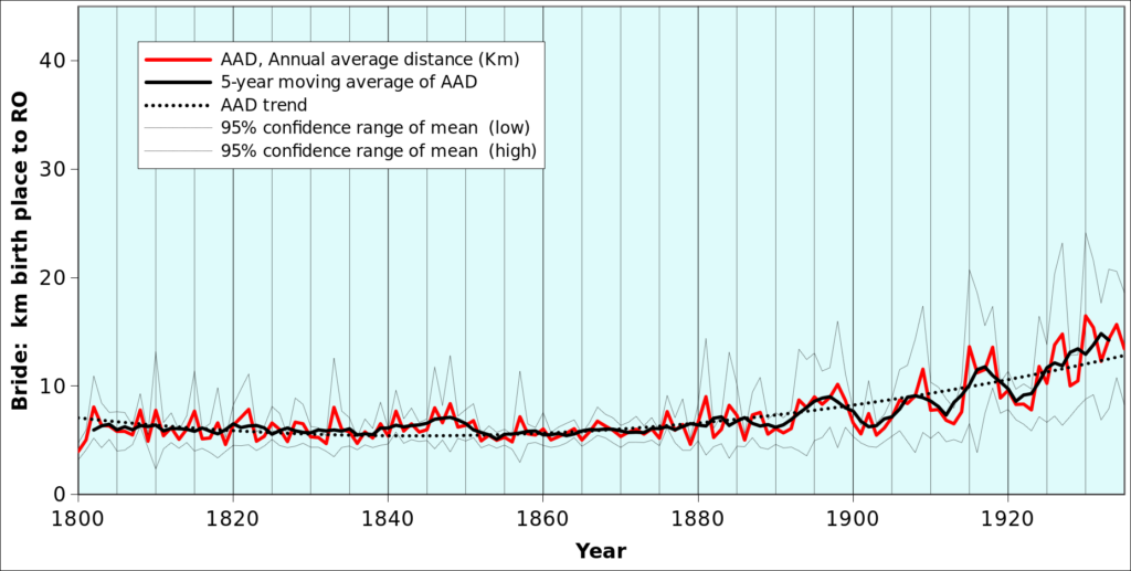
When plotting the average annual values of the distance between the place of birth of brides and locality of the Registry office where they married, figure METHODS-F01 below is obtained((The method outlined in this chapter is illustrated based on the distance between the brides’ s birthplace and the Registry offices (RO). Similar results and conclusions are obtained with grooms and the ROs as well as with the distances between the birthplaces of the spouses)).

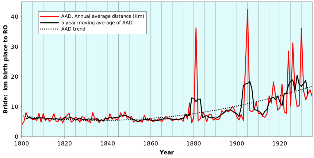
Considering that each point on the red curve is the average of several hundreds of distances, peaks like the one that occured in 1881 or 1905 can only be due a large number of values in the range of 30 to 50 km or, more likely, to one extremely large values like those mentioned in chapter ABSOR.

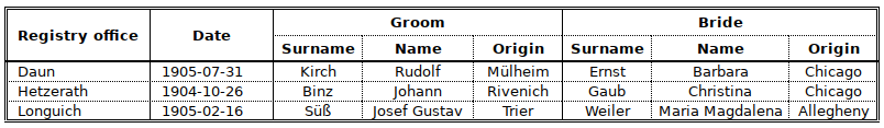
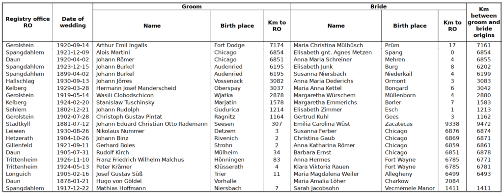
Indeed, the 1905 peak results from the fact that no less than three American women married in the area (Table METHODS-T01). Based on their names, it can be assumed that they are “returning second generation emigrants”. If the listed women are eliminated from the dataset, the averages drop to 6.1 km and 7.1 km for 1904 and 1905)((Additional information and the fulllist of extreme distances are given below in table METHODS-T03)).

METHODS.1.2 About outliers

The averages given in figure METHODS-F01 are “correct” but they are also very misleading because they interfer with longer-term and more fundamental socio-ecomomic trends. Other statistics, such as medians and percentiles as shown, for instance, in table RELOR-T01 are less sensitive to outliers. It remains that it is nevertheless useful to eliminate the outliers from the graphs, among others because less extreme outliers may be more difficult to spot.

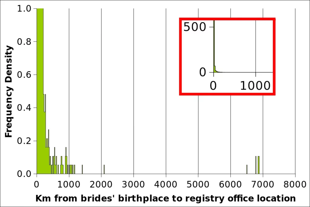
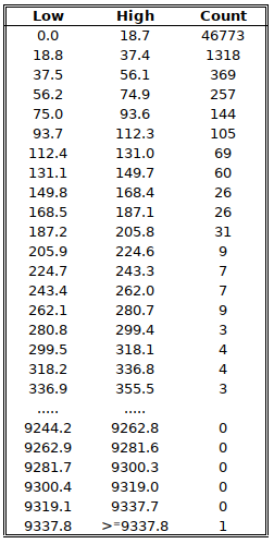
There is a whole science of outliers which, in statistical terms, are data points that differ significantly from other observations. Barbara Ernst, who marries 6851 km from her birthplace (Chicago) is no doubt an outlier (METHODS-T01). The definition of outlier depends on the shape of the statistical distribution of values the outlier comes from. We have stressed repeatedly (e.g. RELOR-T01) that distance statistics are affected by a large skew, i.e. there are many “small” values and some “large” ones. This is very apparent in table METHODS-T02 which shows the thinnning out of the density of observations as the distance increases. It is shown as well in figure METHODS-F02 which displays an extreme zoom into the Frequency density distribution as a function of the distance of brides’ birth places and Registry office. Such a distribution can be seen as a variant of a J-shaped curve, although we are dealing with an extreme case (Refer to Pearson type III curves and the gamma distribution).

It also typically occurs with rainfall in arid places where there is an accumulation of many rainless days with some extremely high records that pull up the mean and cause widespread floods and devastation! In the case of rainfall, there is a large corpus of more or less standard methods. It is generally assumed that rainfall distributions conform to the (Incomplete) Gamma distribution((I have used it throughout my professional life and even wrote about it long ago.I could even make available a scanned copy upon request)).

Let us return to the definition of outliers as “data points that differs significantly from other observations”. There is also the word “significantly” to pay some attention to. If the word is taken in its statistical acception of significance testing, the definition of an outlier will depend on the statistical distribution of the variable. Additional work would be required to find if the actual distribution of distances conforms sufficiently well to one of the mentioned standard distribution, with uncertain outcome.

METHODS.1.3 Identification and elimination of outliers

I mentioned “uncertain outcome” because in heavily skewed distributions, the elimination of the most extreme outlier (largest, in our case) typically leads to the next largest observation to become the next outlier, and this can go on for a large number of data points.

We have, therefore, adopted the following very empirical approach, based on the observation that distances keep increasing over a large range of values, as shown in figure METHODS-F03. When the birthplace to RO distance is plotted against the rank of the observation, the curve increases smoothly over a large range of distances, and then increases abruptly. The values responsible for the abrupt increase have been deemed outliers.

Figures METHODS-F04A and METHODS-F04B are a variant of METHODS-F03 showing only the high end of the curve with the numbering of the ranks in reverse order, i.e. 1 is the highest value, 2 the highest but 1 etc. Based on METHODS-F04B, the 9 largest values were excluded for brides’ birthplace distance to registry office location, the 10 largest for grooms and, logically the 19 largest for the distance between the places of origin of spouses.

The values eliminated are shown in table METHODS-T03 and the resulting revised version of METHODS-F01 appears as METHODS-F05. Except for the confidence interval of the mean, this is the same figure as the one show as RELOR-F01B.