A caveat: all the downloadable files given below correspond to their version on the date of the first publication of this post on 2023-03-03. They are still subject to modification; their final version will be put online at the end of this project.
All the data used in this study are available from this post. They are given in three formats: CSV 1, xlsx2 and Gnumeric, which is the spreadsheet used for this Project.
DATA.1 The complete weddings data set, file BTF (“Big Tonner File”)
This is the final/corrected version the dataset as used in this study, and assembled from files downloaded from the website of KJ Tonner (KJT)
at the end of January 2022. Details are provided in the post entitled 1 – The project database.
The places or origin of the spouses are identified by their “raw names”. Missing fields are left empty.
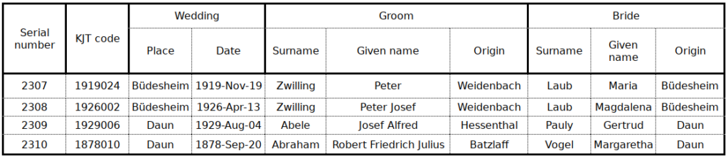
The Serial number was assigned for the purpose of this Project.
Download: BTF_raw.csv.zip , BTF_raw.xlsx , BTF_raw.gnumeric.zip
DATA.2 List of wedding places (“WP File”)
Although the coordinates and the list of wedding places are available from other data files, they are given here in one simple file for the ease of reference. Coordinates are given with six decimals, although the high precision is unnecessary (the 4th decimal corresponds approximately to 1 m at the latitude of the Eifel) .
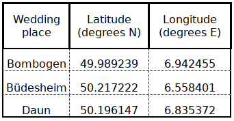
Download: WP.csv
Only the csv file is given as the other formats lead to larger files!
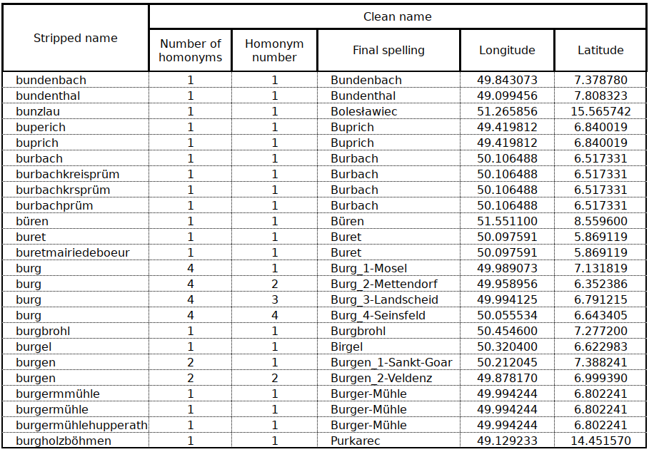
DATA.3 “Stripped” and “clean” names correspondence (“S2C File”)
The table below, which is extracted “as is” from the S2C file illustrates several features
Column 1 has the “stripped name”, which is the slightly modified wedding place name as it appears in the BTF (5.1 above). The number of homonyms is the number of places with the same name. In the case of Burg, we have 4, referred to as Burg_1-Mosel (Burg on the Moselle) , Burg_2-Mettendorf (Burg near Mettendorf), Burg_3-Landscheid (Burg near Landscheid) and Burg_4-Seinsfeld (Burg near Seinsfeld). Each of them has, naturally, different coordinates.
The “clean name” for Bunzlau (a city in south-east Poland, near the Czech border) is Bolesławiec, i.e. the place was renamed from its historical German name to its current Polish name. Buprich, in the municipality of Schmelz, Landkreis Saarlouis in Saarland appears as the correct current spelling (Buprich) but is also mis-spelled as Buperich. Both “stripped names” buprich and buperich are assigned to the “clean” and final variant Buprich. A similar situation arises for (“clean” name) Burger-Mühle which occurs in the BTF as (¨stripped” names) burgermmühle, burgermühle and burgermühlehupperath. Burbach near Prüm occurs in the BTF as burbach, burbachkreisprüm, burbachkrsprüm and burbachprüm, etc.
Without the rather painstaking systematic examination of all individual “stripped” names, it would have been impossible to conduct this study!
DATA.4 Final list of “clean” place names (FC File)
The FC file, in addition to the information in the S2C files, contains additional localities as well as an indicator about the “type” of locality: U (unique), H (homonym), A (average) or TP (Tonner-Pauly, refer to EMIG.2 for details). The specific meaning of the “average” is explained in post 2 – Locating places and sampling the database.
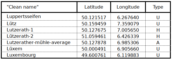
If you have been worrying about the recent eviction of Lützerath to allow the expansion of the Garzweiler coalmine3, note that this happened at Lützerath-2. Lüttzerath-1 is about 100 km further south, and the places with the clean names of Altmühle-Lützerath, Neumühle-Lützerath and Lüzerather-mühle-average are all near Lützerath-1.
Download: FC.csv.zip, FC.xlsx, FC.gnumeric.zip
DATA.5 Prussia 1881 shapefile
The file was prepared based on the shapefile published in the Cshapes project of the Center for Comparative and International Studies, Department of Humanities, Social and Political Sciences, ETH Zurich. Compared with the original file, Ostbelgien and the so called “Prussian Walloonia” were added and the level of detail (1:1 million scale) was increased on the western border from Alsace, Lorraine, Luxembourg and Belgium.
Download: Prussia 1881 shapefile
DATA.6 Environmental data
The environmental data stem from various published sources that are described in the chapter on Environmental variables. Additional info and meta-data, as well as details of the processing will eventually be added in the files once they reach “maturity”. There are currently three environmental data sets available:
The csv file includes scPDSI (Self-calibrating Palmer index); FracCrop and FracPast, the fraction of cropland and the fraction of pastures; seasonal and annual rainfall Rain_MAM, Rain_JJA, Rain_SON, Rain_DJF, Rain_year; seasonal and annual temperature Temp_DJF, Temp_MAM, Temp_JJA, Temp_SON and Temp_year.
The csv file includes the same data as the previous file, but “normalised”, i.e. the variables are expressed as standard deviations departure from the 1853-1888 average.
This data set is derived from Environmental-data_actual_rounded above.
DATA.7 Gemeindelexikon (“Municipal Encyclopaedia”) and 1885 census results for the Rhineland province
The downloadable document contains only the pages that are relevant for the current Project. The original document is entitled
Gemeindelexikon für das Königreich Preußen. Auf Grund der Materialien der Volkszählung vom 1. Dezember 1885 und anderer amtlicher Quellen bearbeitet vom Königlichen Statistischen Bureau. XII. Provinz Rheinland. Berlin SW: 1888. Verlag des Königlichen Statistischen Bureaus.
It is downloadable from various repositories of historical German documents, such as the Zeitschriften Datenbank or the Statistische Bibliothek.
DATA.8 Detailed 1885 digital census data for the Registry Office Districts (Standesamtbezirk)
The relevant information in the Gemeindelexikon (5.7 above) was scanned and is provided as a downloadable csv file. The file contains the land-use and population details for all the all Rural communities (Landgemeinden, villages) mentioned in Chapter 7 (Number of weddings year by year).
DATA.9 Gridded data of the number of spouses per pixel
The file was interpolated using Shepard’s method as implemented in Jürgen Grieser’s New_LocClim software. A description of the tool as well as the software itself are available from the author’s website. 2346 data points were mapped to a 0.05° x 0.05° degree grid between longitudes 1°E and 26°E and latitudes 42°N and 58°N. The estimated spatial average is 1.68. The Data point based error estimates are Bias=-7.73, Variance=343.8 and RMS=343.9; the grid based error estimates are Bias=-0.03, Variance=20.04 and RMS=20.04. All units are counts of spouses.
The resulting downloadable file is Number-of-spouses-per-pixel_shepard_3_na.csv. Values that could not be interpolated are codes as “na”.
The comma-separated file contains, for each line, Longitude and latitude at 0.05 degree intervals and the number of spouses. An example is given below:
22.35,57.65,1
22.35,57.7,1
22.35,57.75,na
22.35,57.8,na
22.35,57.85,na
22.35,57.9,na
22.35,57.95,na
22.35,58,na
22.4,42,1
22.4,42.05,1
22.4,42.1,1
22.4,42.15,1
22.4,42.2,1
22.4,42.25,1
22.4,42.3,1
Here is some additional information about Shepard’s method taken from the Help of New_LocClim software. Although the method is especially designed for climate interpolation, it provided the best interpolation of the number of spouses data. Below, “data points” correspond to 3 numbers: the coordinates of a locality (llatitude, longitude) and the number of spouses that originate in this locality, as in the example above.
First a circle is drawn around the grid point containing, on average, seven data points. If there are less than four or more than ten data points within the circle the radius is changed so that the fifth nearest or the eleventh nearest data point lies on the frame of the circle. This procedure ensures that the length scale is taken as a constant. Only in regions with very high or very low data point density is the scale changed to keep the number of data points used for the interpolation between four and ten. Within the circle a weight function is applied which monotonically decreases with the radius.
In the next step the weights are altered with respect to a directional isolation of the data points. This step is like a simple shadow correction.
Since the weight function itself is like inverse distance weighted averaging in the close vicinity of a grid point, it would lead to singular points if a grid point and a station location coincide. Even if they do not coincide but lay close together, the grid point may become a unreasonable local maximum or minimum just because the closest data point has an extraordinarily high weight. This situation is avoided by using a small local average-gradient correction where no data point is very close to the data point with respect to grid size. Finally, if one or more data points are very close to a grid point the simple average of these data points is taken as the interpolated value.
One further advantage of Shepards Method is that it runs completely automatically. No parameters have to be set. It automatically takes station density and grid size into account.