This chapter on environmental variables provides some background about weather/climate conditions under which the Eifel weddings took place. While it is difficult to determine if other factors than love and tradition played a part, it is logical to assume that politics and weather may, to an unknown extent, have affected the spatial and temporal patterns of weddings when long periods are taken into account. This section provides some backgroud information that may prove relevant.
The years covered in this study, 1800 to 1935, span a period that, in many ways, constitutes the transition from the old, mostly unmechanised Ancien régime to the area of machines, steam engines and the development of the chemical industry (including chemical fertilisers). It is also the time when Prussian educators invented the modern school which was almost universally adopted. The German confederation (1814-1866) witnessed an explosion of interest in technical and scientific matters including, of course, meteorology and geology.
Introduction
The 1850s are usually considered the beginning of the Instrumental temperature record, i.e. thermometers had reached a sufficient degree of standardisation and reliability to produce readings that allowed to compare different times and different locations. A raingauge (or pluviometre), on the other hand, is a significantly less sophisticated instrument. Its simplest form is a bucket that, as long as it is not located under a tree, will produce useful readings.
Both rainfall and temperature started to be recorded systematically around 1850 by ad hoc organisations: the Royal Meteorological Society was established in 1850, the Königlich Preußisches Meteorologisches Institut in Berlin goes back to 1847, but because of the diversity of States that made up Germany at the time, many regional efforts were uncoordinated. In fact, the German weather Service (Deutscher Wetterdienst, DWD) was formally established only in 1952. It is stressed, however, that as early as the 1780s, the Societas Meteorologica Palatina, also referred to as Mannheimer Meteorologische Gesellschaft organised systematic international weather observations throughout Europe. The Hohenpeißenberg Meteorological Observatory has a continuous temperature record since 1781.
There are also numerous “private” series of meteoeorological observations, e.g. those of Johannes Löh (born in Benningshausen, 51.654045N, 8.240535E), as well as large collections of anecdotal observations of extreme events (including by the current writer: Gommes, 1980).
As a result of the diversity of measuring techniques, locations, duration of records etc, it is very difficult to establish homogeneous time series for specific areas before the Instrumental period was fully established. In the transition period, which almost exactly coincides with the years covered by this project, proxies have to be relied on, for instance for the area in the current Project hull. Depending on the time scale, other techniques and sources of data can be resorted to, notably tree ring analyses, which are the object of dendrochronology and dendroclimatology, i.e. the reconstruction of environmental conditions based on tree growth 1.
How to understand the reconstructed “climatic” variables
There are many reconstructions of historical weather to well before the instrumental period (see the References below, which include the sources listed in the next table, in addition some generic references).
For the present study, we have adopted readily available published data corresponding to a rectangle larger than the Project hull, referred to below as the “Climatic square”.
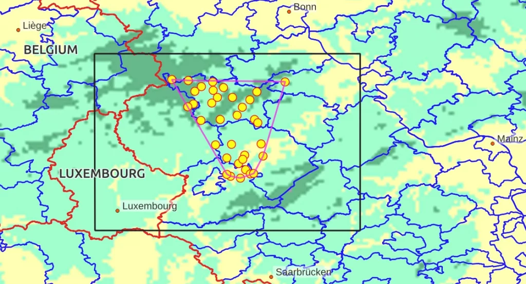
The “Climatic square” (6.0 E to 7.5 E and 49.5 N to 50.5 N)Cis approximately 107 km across (W to E) and 111 km from N to S. It includes 1210 localities (49% of the total) ; 93% of all spouses originate from inside the “climatic square” 2.
The Dutch national weather service (KNMI, officially “Royal Netherlands Meteorological Institute” ) maintains a server (the KNMI climate explorer i) from where a number of publicly available data can be downloaded.
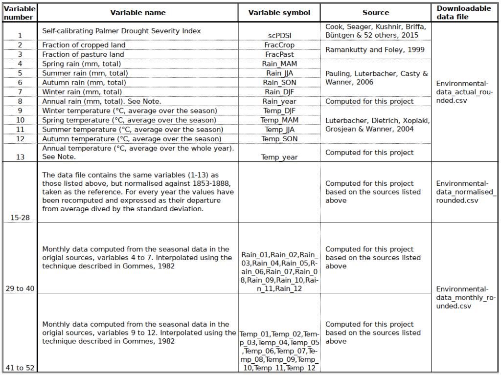
For the present project, the following data were downloaded covering the period 1791 to 1935 and average over the Climatic square:
A word of explanation about scPDSI
All the variables in the table are well known and immediately understandable.
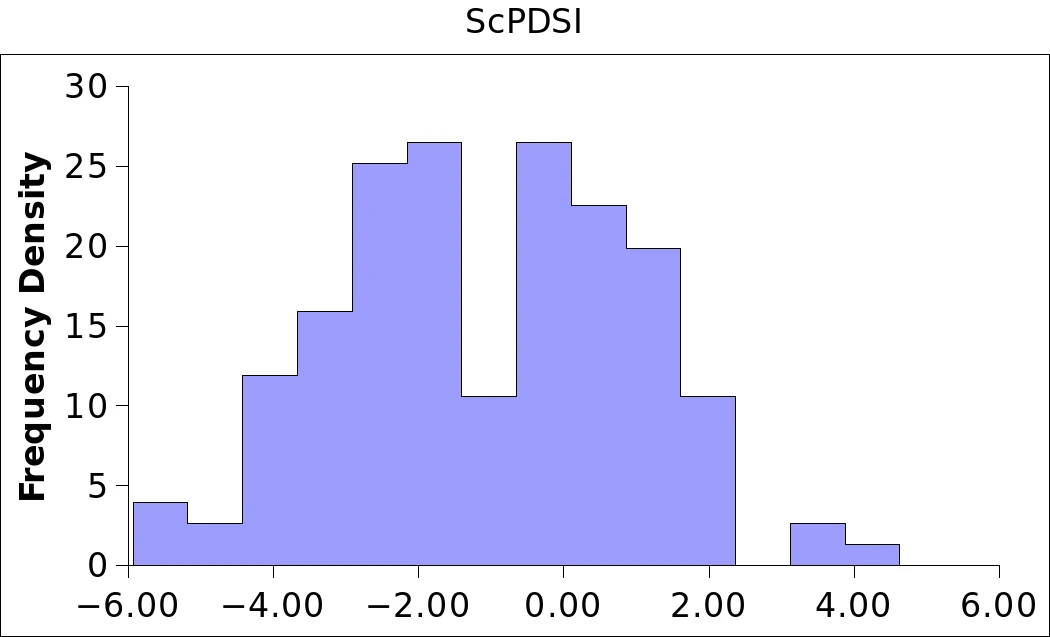
The self-calibrated (or self-calibrating) Palmer Drought Severity Index (scPDSI) needs a word of explanation. The index spans the values from -10 (extremely dry) to +10 (extremely wet) but usually remains within the -4 to +4 range (see histogramme below). Originally known as PDI, Palmer Drought Index, it is a classical drought monitoring tool that has constituted the basis of weather monitoring for agriculture in the US since the mid 1960s.
It was originally computed with weather station data and is based on a soil water balance (SWB). A SWB works as follows: for successive monitoring intervals (e.g. weeks), it is considered that crop available water is the sum of soil moisture plus rainfall. Crops consume water at a rate that is a function of atmospheric water demand 3 and the water left over at the end of the monitoring interval is available for the crop at the beginning of the next monitoring interval. Since PDSI measures the biological impact, and since dendrochronology also measures impact, there is, in theory, a direct compatibility between the two technical fields.
The self-calibrated variant of PDSI (scPDSI) was proposed in 2004 by Wells, Goddard and Hayes to improve the spatial representativeness of PDSI, making assessments in different climate zones more compatible. The original paper can be downloaded here.
And another word about winter data
The reader may have noticed that, for rainfall, the seasons are given as MAM, JJA, SON, DJF, while for temperature we have DJF, MAM, JJA and SON. In other words, for rainfall winter is at the end of the year, while for temperature it is at the beginning. Since a calendar year actually has two winters the two options are indeed possible. However, the only option that makes sense, from a biological and agricultural point of view is DJF, MAM, JJA and SON because the Eifel does grow winter crops and summer crops, and it is the conditions of the previous winter that matter!
The table of variables list annual rainfall and temperature. The values are not provided by Pauling et al. and by Luterbacher et al. Actually, they were computed by redistributing Rainfall and Temperature to the respective years, e.g. 2/3 of the previous year’s winter rain was assigned to the current year, as well as 1/3 of the current years winter precipitation.
Heavy processing makes lazy variables4
As already mentioned, all environmental variables in this Project are proxies, i.e. derived based on indirect evidence5. It is also stressed that all climatological processing reduces the variability that occurs in the real world6. This is even more so when statistical methods are used to calibrate time series and when some spatial average are involved, as is the case for the climatic square. The data published in the listed sources are all grids, i.e. pixel-based “images”. In order to extract the data for the Climatic square, pixel data had to be further averaged or otherwise combined. The number of data underlying the Square averages depends on the spatial resolution of the original data and differs for the different variables.
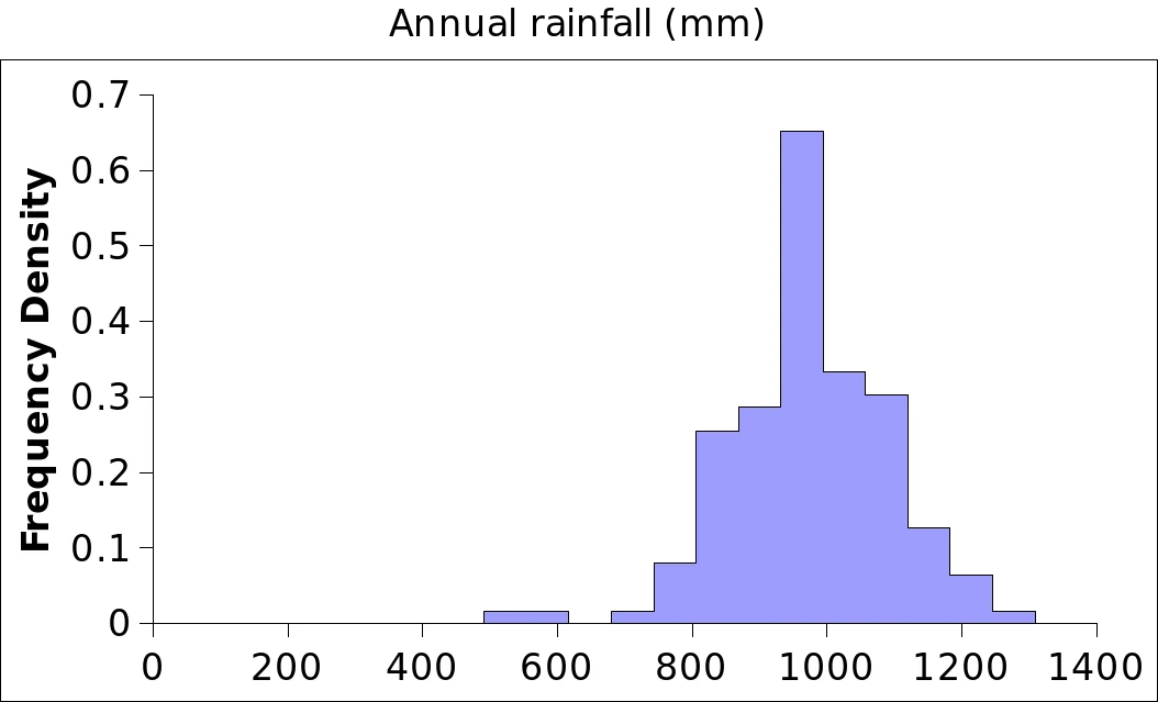 | 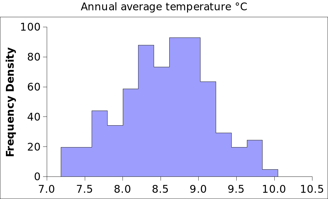 |
 |  |
 | VARENV – F02 a b c d e – Some sample histogrammes corresponding to the assembled time series |
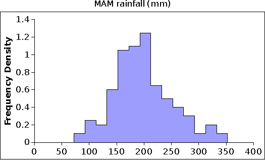
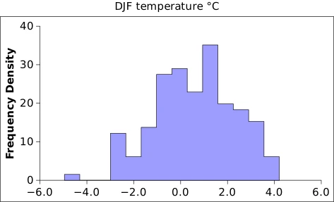
The statistical distribution of the climate variables over the Climatic square is untypically well behaved and rather symmetrical. Real world variables are much more difficult to handle, e.g. with large positive skewness in rainfall most of the time. The fluctuation interval is also very narrow, for instance. The biomodal histogramme for scPDSI is very unusual. It looks as if we had two populations, and this seems indeed to be the case: a relatively dry period up to 1845, and wetter conditions thereafter (refer to the third “colourful time series graph” below). Logically, since scPDSI is based on Rain and Temp, the change should also be reflected in those variables7.
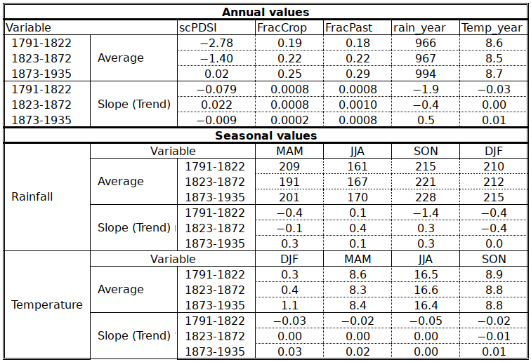
In order to determine whether the time series can indeed be subdivided into three different periods (1791-18228, 1823-1872 and 1873-1935), the following table was prepared to show averages and trends over the respective periods. None of the climate variables shows any significant difference between the periods at the 0.05 confidence level. However, scPDSI and land cover fractions do display a marked trend with the result that the average between the 1791-1822 and 1873-1935 periods are significantly different at the 0.01 level, even at the 0.001 level for scPDSI. This is puzzling and will need some additional exploration.
Some statistical features of the complete time series
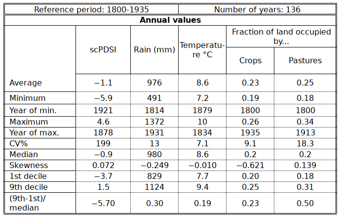
The tables and the figures below summarise the environmental statistics over the “Climatic square” for the whole period (1800 to 1935). It is stressed that for the land-use fractions, being basically linear (see last figure) most of the statistics make little sense (e.g. the coefficient of variation). For each of the variables, the extreme values are indicated, together with the year during which the extremes occurred. More detailed information can be found for variables in the chapter HIST of Moving boundaries, where the changing political landscape is taken into account.
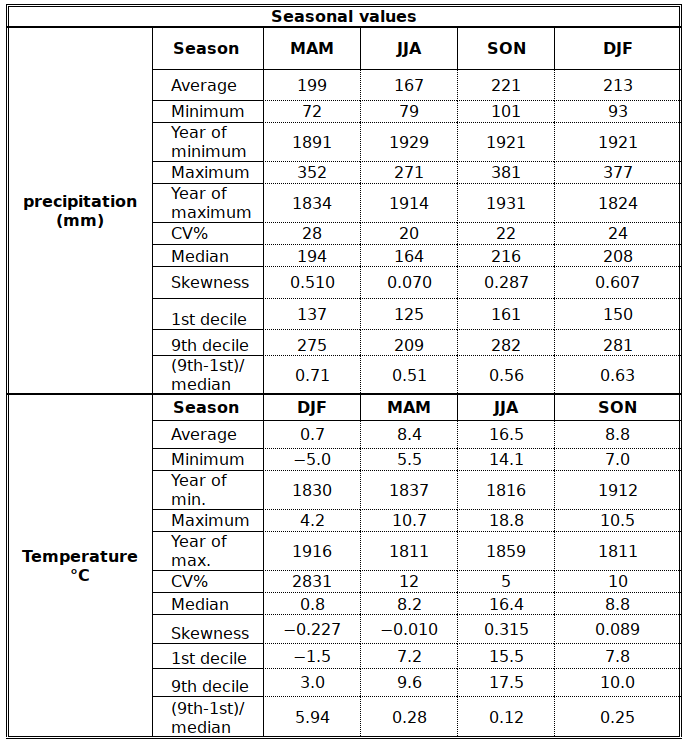
Compared with the tables in the HIST chapter the current chapter adds a list of statistics that all aim at assessing the amount of variability and the level of symmetry in the data’ s distribution. As already mentioned, scPDSI is significantly more variable than all the other variables. The rainfall data, including seasonal ones, are – again – rather dull. They are slightly more variable than temperature, with the exception of winter temperature, which clearly emerges as the season with the largest inter-annual variability. If the data are to be trusted, it is winter that puts its stamp on a year and makes it different. NW Europe is one of the regions in the word with the largest relative excess of rainfall over Evapotranspiration9. As a result, a 50% drop in precipitation is usually not catastrophic. On the contrary, there are several recent examples in Europe when “drought” resulted in bumper harvests because of the unusually favorable sunshine.
The variables in the time series are, naturally, not independent. A handful of correlations reach about 0.5. Seasonal rainfall values tend to be uncorrelated among themselves, except SON and MAM with total annual rainfall. Temperatures, on the other hand, are inter-correlated, indicating a lot more persistence than for rainfall: years are either cold or warm throughout. The most interesting correlations are the ones illustrated below.
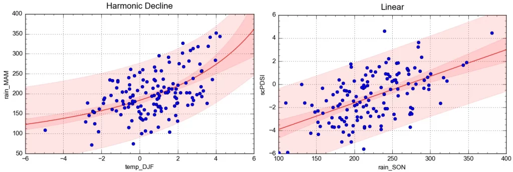
The first graph says basically “cool winter, wet spring”, which seems to agree with popular wisdom. This would need to be assessed in terms of agricultural impact as it may also mean “poor winter crop.” The second graph makes sense and lends credibility to the scPDSI values.
Some colourful time series graphs
The series of colourful time series graphs that follow were designed in such as way that individual years can be identified. The years are supposed to be calendar years (Jan to Dec), in line with the tradition of climatologists, and to ensure that rainfall and temperature refer to the same period.
The main use of the graphs will be in the chapter analysing the variability of the number of weddings.
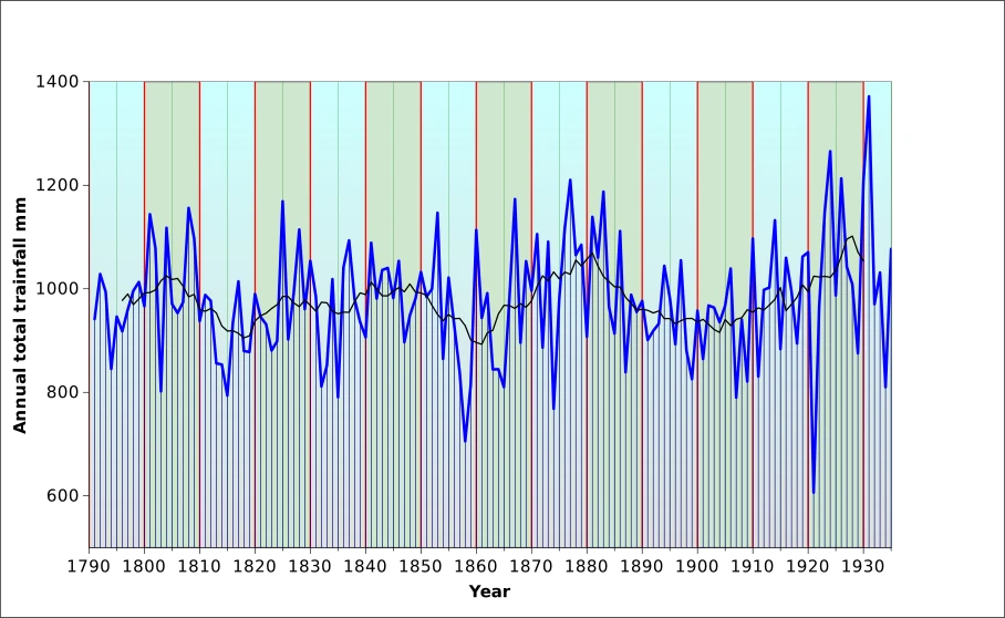
The graph shows regular fluctuations which, on the moving averages curve, seem to be vaguely pseudo-periodic. with variability increasing significantly from WWI, but both the wettest year (1932, with 1372 mm) and the driest one (1921, 606 mm). The same years were also the coolest and the warmest, respectively. The behaviour is reflected in the seasonal values which indicate that it was the second half of the years that was most anomalous. In the 19th century, the driest and the wettest years were 1858 and 1877.
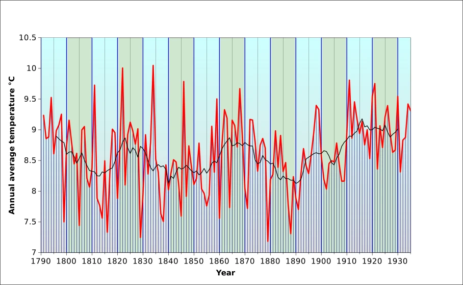
The temperature curve appears more chaotic that the rainfall pattern. And contrary to rainfall, interannual variability was largest approximately between 1810 and 1850, with marked high values in 1811, 1822, 1834 and 1846. The four lowest values are those of 1879, 1888, 1829 and, naturally 1816, the “year without a summer”, which was a hemispheric phenomenon and is well documented. One of the first widely available accounts was published by Stommel and Stommel in the Scientific American in 1979. At the “micro” scale, and directly relevant for the Eifel, we could mention Conrads (1938) who describes the situation in Lammersdorf (50.633567 N, 6.275476 E) during the spring of 1817: instead of harvesting grass, nettles, clover and other herbs for cattle, they were cooked and mashed to feed hungry families. Hunger forced many people to emigrate. Conrads and other sources also mention high prices of food and shortage of seeds, which carried over the famine into the next year.
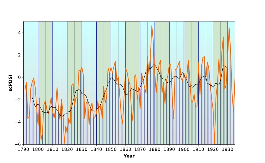
The scPDSI was already referred to repeatedly at the beginning of this chapter. More clearly than the other curves, it shows several runs of drought years, as during 1802-1803, 1818-1820, 1832-1844, though this period had less severe drought than the ones mentioned previously. If the scPDSI is to be trusted, the most severe droughts happened in 1818 and, almost exactly a century later, in 1921.
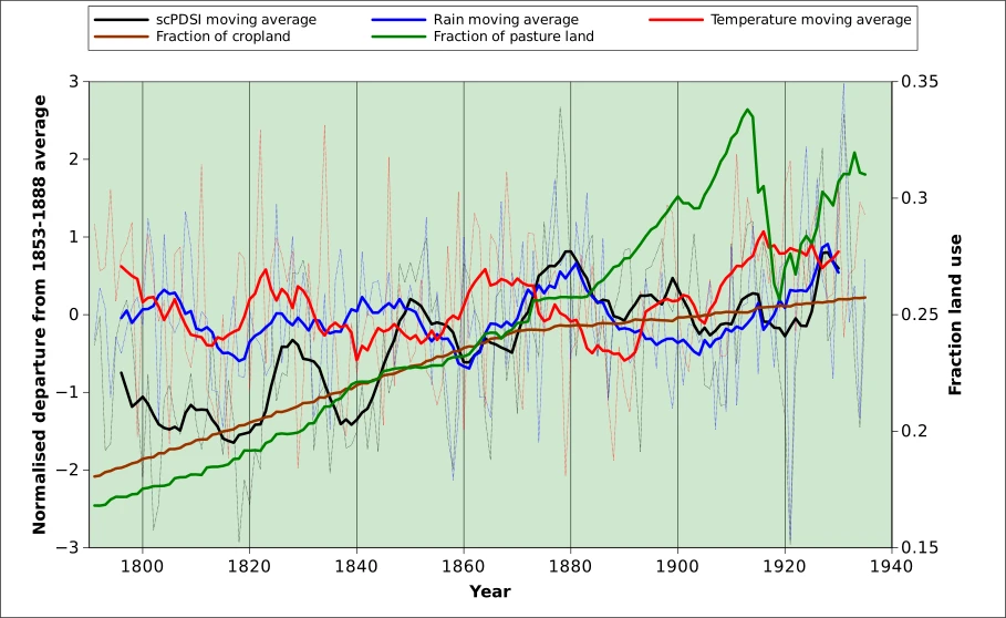
The last graph (below) shows normalised values, i.e. they are expressed as departures (number od standard deviations) from the 1853-1888 average. Purely impressionistically, the graphs shows some synchronisation between rainfall, temperature and the resuting scPDSI up to approximately 1860. After a priod of diverging patterns, the curves roughly synchronise again after 1900. Neddless to say, the land use curves follow the own logic where the war economy plays a dominant role.
References
Büntgen U, V Trouet, D Frank, H H Leuschner, D Friedrichs, J Luterbacher & J Esper. 2010. Tree-ring indicators of German summer drought over the last millennium. Quaternary Science Reviews 29 (2010) 1005–1016
Büntgen U, W Tegel, K Nicolussi, M McCormick, D Frank, V Trouet, J O Kaplan, F Herzig, K-U Heussner, H Wanner, J Luterbacher, J Esper. 2011. 2500 Years of European Climate Variability and Human Susceptibility. Science 331:578-582
Casty C, C C Raible, T F Stocker, H Wanner & J Luterbacher. 2007. A European pattern climatology 1766–2000. Clim Dyn 29:791–805.
Conrads J. 1938. Das Venndorf Kalterherberg mit dem Kloster Reichenstein. Aachen, Verlag Johannes Volk. 290 pp.
Cook, E R, R Seager, Y Kushnir, K R Briffa, U Büntgen & 52 others. 2015. Old World megadroughts and pluvials during the Common Era. Sci. Adv. 1, e1500561.
Dobrovolný P, A Moberg, R Brázdil, C Pfister, R Glaser, R Wilson, A van Engelen, D Limanówka, A Kiss, M Halíčková, J Macková, D Riemann, J Luterbacher & R Böhm. 2009. Monthly, seasonal and annual temperature reconstructions for Central Europe derived from documentary evidence and instrumental records since AD 1500. Climatic Change DOI 10.1007/s10584-009-9724-x 35 pp
Esper J, D C Frank, M Timonen, E Zorita, R J S Wilson, J Luterbacher, S Holzkämper, N Fischer, S Wagner, D Nievergelt, A Verstege & U Büntgen. 2012. Orbital forcing of tree-ring data. Nature Climate Change 2: 862-866
Gommes, R., 1980. Die Wetterlage in Laufe der Zeit, samt einer Beschreibung des
Katastrophenjahres 1740 aus dem Pfarrarchiv Reuland. Part 1. Zwischen Venn und Schneifel,
(15) : 162-166, part 2. Z.V.S (16) : 188-191.
Gommes, R., 1983. Pocket computers in agrometeorology. FAO Plant production and protection
paper N. 45, FAO, Rome, 140 pages.
Herget J & H Meurs. 2010. Reconstructing peak discharges for historic flood levels in the city of Cologne, Germany. Global and Planetary Change 70 (2010) 108 et sq.
Lamb, H.H. 1982. Climate, history and the modern world. Methuen. London and New York. 387 pp.
Ljungqvist F C, A Seim, H Huhtamaa. 2021. Climate and Society in European history. WIREs Clim Change 2021; 12:e691 28 pp
Luterbacher J, D Dietrich, E Xoplaki, M Grosjean & H Wanner. 2004.European Seasonal and Annual Temperature Variability, Trends, and Extremes Since 1500. Science 303:1499-1503. Data downloaded from https://climexp.knmi.nl/start.cgi.
National Research Council. 2006. Surface Temperature Reconstructions for the Last 2,000 Years. Washington, DC: The National Academies Press. 160 pp. Committee on Surface Temperature Reconstructions for the Last 2,000 Years, Board on Atmospheric Sciences and Climate, Division on Earth and Life Studies. https://doi.org/10.17226/11676. Downloadable from http://nap.nationalacademies.org/11676
Pauling A, J Luterbacher J, C Casty C & H Wanner. 2006. Five hundred years of gridded high-resolution precipitation reconstructions over Europe and the connection to large-scale circulation. Clim Dyn 26:387–405
Ramankutty N & J A Foley. 1999. Estimating historical changes in global land cover: Croplands from 1700 to 1992.Global Biogeochemical cycles, 13(4):997-1027.
Stommel H & E Stommel, 1979. The year without a summer. Scintific American 240(6):176-186
Wells, Nathan & Goddard, Steve & Hayes, Michael. (2004). A Self-Calibrating Palmer Drought Severity Index. Journal of Climate – J CLIMATE. 17. 2335-2351. 10.1175/1520-0442(2004)017<2335:ASPDSI>2.0.CO;2.
Wetter O. 2017. The potential of historical hydrology in Switzerland. Hydrol. Earth Syst. Sci., 21, 5781–5803
- Data from trees that grew during the instrumental period can be used to calibrate dendrochronological data, i.e. assuming that the same factors cause the same effects, features of tree growth prior to the instrumental period are explained by the same known factors that caused them during the instrumental period.[↩]
- The “square” appears as a rectangle due to the projection[↩]
- Potential evapotranspiration, based on a simplified method involving just temperature[↩]
- They lose their variability and tend to concentrate near the average; as a result, they typically make for optmistic impact assessments[↩]
- For instance, what I call “rain” is in fact a “rain equivalent”, a modeled spatial equivalent of rain, etc.[↩]
- This applies as well to projected future weather![↩]
- Note however, that the Cook scPDSI series is essentially tree-ring based. If the “inflexion” around 1845 is also present – statistically speaking – in the other time series, there may be some reality in the phenomenon.[↩]
- 1791 was preferred over 1800 in this case to add some statistical weight to a period that would otherwise have been very short[↩]
- Statistically speaking, this qualifies the climate as “extreme”.[↩]