As I was updating a couple of things in another corner of this blog,  I stumbled upon of  a passage in a recent book by Nate Silver (2012) that has a lot of relevance for crop forecasters. It is relevant to two different but related subjects: (1) averaging different forecasts and (2) mixing cross-sectional data (belonging to different spatial units) with time-series data. The subject keeps coming up, and not later than last week, Wolfgang wrote in an email  Are there really “reliable methods to determine risk when limited time depth is available?” Except, perhaps, by substituting space for time, a conceptually doubtful approach.  He also said, quite rightly, that Spatial interpolation should in not be called “averaging”

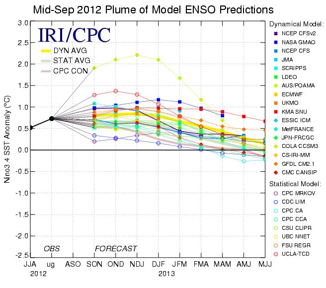
ENSO (El Niño Southern Oscillation) predictions by about 25 different laboratories. “About 25” because many of the above institutions are linked and share methodologies. Source of figure: http://www.srh.noaa.gov/bmx/?n=elnino

The reality is, that consciously or inconsciously, we keep crossing the boundary between spatial and temporal data all the time. Take satellite-based rainfall estimates (see this post for examples). They mix ground rainfall (point location with time-continuous reading of limited spatial validity) with cloud indices (a spatial average over an area much larger than the one covered by a raingauge, but time-discontinuous: the satellite looks at the clouds every 15 or 30 minutes only). Both the raingauge and the satellite provide proxies for a variable we don’t know: average spatial rainfall, which, in turn, can be obtained using other approximations: geostatistics and modelling (Gommes, 1993). What about crop yield estimates based on satellite imagery (by pixels), ground data from weather stations (points) and agricultural statistics by province? If it’s not a mix, it’s a mess. Yet, those methods do work (Balaghi et al 2012). What about the El Niño forecasts that are issued regularly by many laboratories worldwide. As they cannot easily be averaged, you will come across statements saying “there is a 30 % chance that we are heading for El Niño conditions”, when in reality none of the predictions does say that. It is just that 30 % point in one direction (El Niño) and 70 % point in another direction (Neutral or La Niña). Really, this is not the same as saying “there is a 30 % chance”, because the forecasts are not independent (they use similar methodologies and largely the same data) and their forecasting skill is different (some have a better record than others), so that -if we should average – not all predictions should have the same weight.

Forecasters frequently refer to a “method” which they call “convergence of evidence”. Out of curiosity, I looked it up on Wikipedia, where I found that In science and history, consilience (also convergence of evidence or concordance of evidence) refers to the principle that evidence from independent, unrelated sources can “converge” to strong conclusions. Does it apply to our case? If we agree that our data sources are “independent” and “unrelated”, we could… but they are not!

Let me take another final example. There has been a lot of research on rainfall estimation in Africa (Beyene and Meisner 2009, Dinku et al 2007, Funk et al 2003, Grimes and Pardo-Iguzquiza 2010, Rojas et al 2011). Many institutions monitor African crops, using as their primary input a combination of ground data (rainfall) and satellite information (cloud cover) known as RFE (Rainfall Estimate). RFE is provided by the website of the NOAA Climate Prediction Center and by some other sources (Note 1). The methodology is described in detail by various links on the mentioned webpage. Even some national meteorological services (I won’t mention which!) find it easier to use RFE than their own data, which are often missing, difficult to use because of exotic formats etc. Altogether, RFE is this is thus a very useful service provided to the community. However, what would happen if, for some reason, the algorithms undelying RFE did not provide accurate results in, say, July 2013? All the national and international crop condition assessments using RFE would be wrong. Needless to say, this is another strong point in favour of the multiplication of independent data sources, and for the averaging of forecasts based on independent data. Rainfall from the meteorological network and NDVI, for instance, provide independent data sets and indicators…

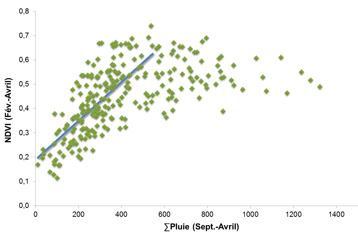
A graph mixing cross-sectional and time series data: average February to April NDVI (NOAA-AVHRR) in Moroccan cropped areas as a function of September to April rainfall. The 345 points in this figure represent data from 23 weather stations for the years 1990 to 2004. Source: fig. 40 in Balaghi et al, 2012.

The reality of ground data is often such that  the mixing of cross-sectional and time-series data is the only way we have to “increase” data available for calibration (e.g. 12 years in 5 neighbouring districts = 60 data items). This can give us at least some confidence in a calibration, in the sense that it can be shown very empirically that the mix is reasonably homogeneous, and therefore acceptable as a basis for calibration and forecasting. For instance, we can randomly split the data into two batches of 30 and verify that we get similar coefficients in the two batches, or we can take the “old” years and compare them with the “recent” ones and verify that, there too, coefficients are comparable (Of course, everything that needed detrending has been detrended beforehand.)

I am, at good last, coming back to Silver. Here is the passage I mentioned above: Nevertheless, there is strong empirical and theoretical evidence that there is a benefit in aggregating different forecasts. Across a number of disciplines, from macroeconomic forecasting to political polling, simply taking an average of everyone’s forecast rather than relying on just one has been found to reduce forecast error,14 often by about 15 or 20 percent. But before you start averaging everything together, you should understand three things. First, while the aggregate forecast will essentially always be better than the typical individual’s forecast, that doesn’t necessarily mean it will be good. For instance, aggregate macroeconomic forecasts are much too crude to predict recessions more than a few months in advance. They are somewhat better than individual economists’ forecasts, however. Second, the most robust evidence indicates that this wisdom-of-crowds principle holds when forecasts are made independently before being averaged together. In a true betting market (including the stock market), people can and do react to one another’s behavior. Under these conditions, where the crowd begins to behave more dynamically, group behavior becomes more complex. Third, although the aggregate forecast is better than the typical individual’s forecast, it does not necessarily hold that it is better than the best individual’s forecast. Perhaps there is some polling firm, for instance, whose surveys are so accurate that it is better to use their polls and their polls alone rather than dilute them with numbers from their less-accurate peers. When this property has been studied over the long run, however, the aggregate forecast has often beaten even the very best individual forecast. A study of the Blue Chip Economic Indicators survey, for instance, found that the aggregate forecast was better over a multiyear period than the forecasts issued by any one of the seventy economists that made up the panel. (Kindle Loc. 5657-73)

A note in the passage refers to the paper by Bauer et al (2003), which is well worth looking at by agrometeorologists and remote sensers. It appears that economists do not only compute ratios of percentages and say “ex post” and “ex ante” all the time, they also use cross-sectional data for tuning models.

And we should not hesitate to do the same!

Notes

(1) Here are three additional sources of rainfall estimates over Africa: the TAMSAT group at the university of Reading, IRI and and FAO. Do drop a line to FAO to complain about a useful site that has not been updated since 2010, losing customers and credibilty at the same time. O tempora o mores!

References

Balaghi R, Jlibene M, TYchon B, Eerens H 2012 La prédiction agrométéorologique des rendements céréaliers au Maroc. INRA, Maroc, 153 pp. This is a little book that many aspiring and seasoned crop forecasters should read: It is full of ideas, standard and not-so-standard methodst that can use to extract yield information from remote sensing and ground data. It can be downloaded (in French) from the website of INRA: click here. An English version is also available.

Bauer A, Eisenbeis RA, Waggoner DF, Tao Zha 2003 Forecast Evaluation with Cross-Sectional Data: The Blue Chip Surveys. Economic Review, Federal Reserve Bank of Atlanta, 2003. http://www.frbatlanta.org/filelegacydocs/bauer_q203.pdf.

Beyene EG, Meissner B 2009 Spatio-temporal analyses of correlation between NOAA satellite RFE and weather stations’ rainfall record in Ethiopia. Int. J. Appl. Earth Observ. Geoinform. (2009), doi:10.1016/j.jag.2009.09.006

Dinku T, Ceccato P, Grover-Kopec E, Lemma M, Connor Sj, Ropelewski F 2007 Validation of satellite rainfall products over East Africa’s complex topography, International Journal of Remote Sensing, 28:7, 1503 – 1526 To link to this article: DOI: 10.1080/01431160600954688, URL: http://dx.doi.org/10.1080/01431160600954688

Funk C, Michaelsen J, Verdin J, Artan G, Husak G, Senay G, Gadain H, Magadazire T 2003 The collaborative historical african rainfall model: description and evaluation. Int J Climatol 23:47–66

Gommes, R. 1993. The integration of remote sensing and agrometeorology in FAO. Adv. Remote Sensing, 2(2):133-140.

Grimes D, Pardo-Iguzquiza E 2010 Geostatistical analysis of rainfall Geograph Anal 42:136–160.

Rojas O, Rembold F, Delincé J, Léo O 2011 Using the NDVI as auxiliary data for rapid quality assessment of rainfall estimates in Africa, International Journal of Remote Sensing, 32:12, 3249-3265 (http://dx.doi.org/10.1080/01431161003698260)