TYPOL.1 Purpose

A number of environmental and population-related variables have been collected in the ambit of Chapters LUCLIM, VARENV and WEDNUM. They can be used to define a typology of the Registry office districts (Standesamtbezirk).

Only “concentrations” were retained, thus excluding variables that depend on the size of the districts (“intensities”, e.g. district areas or population numbers). Such variables are very inter-correlated and tend to dominate numerical classifications at the expense of the finer detail of “concentrations” contained in ratios like population density and the wedding rate. The ratios are scale independent and contain a marked qualitative component .

The variables were used to group (cluster) Districts which are qualitatively similar and therefore systematically identify similarities and differences between the Districts. This typology can be used to understand systematic differences in the statistics and geostatistics of the marriages.

TYPOL.2 List of available variables

[01] Geo_Lat, Latitude in decimal degrees;
[02] Geo_Lon, Longitude in decimal degrees;
[03] Geo_Alt, Altitude in m. above sea level as obtained from the ETOPO grids((Amante, C. and B. W. Eakins, ETOPO1 1 Arc-Minute Global Relief Model: Procedures, Data Sources and Analysis. NOAA Technical Memorandum NESDIS NGDC-24, 19 pp, March 2009.));
[04] Clim_Rain Rainfall, 1961-90 average (interpolated based on DWD stations: cf. Chapter LUCLIM.2)
[05] Clim_Temp Temperature, 1961-90 average (interpolated based on DWD stations: cf. Chapter LUCLIM.2);
[06] Vill_num, Number of Villages (Landgemeinden) covered by the Registry office district (Standesamt) and available from chapter DATA.8. It is stressed that the variable is not scale dependant;
[07] Vill_Ha, Average area of Villages (refer to Number of “Rural communities” in chapter WEDNUM.2 and chapter DATA.8);
[08] Vill_Pop, Average population of villages (refer to chapter WEDNUM.2, number of “Rural communities” and Chapter DATA.8);
[09] LU_crop_pc, Percentage of land used for cropping (refer to chapter WEDNUM.2);
[10] LU_pasture_pc, Percentage of land used for grazing area (refer to chapter WEDNUM.2);
[11] LU_wood_pc, Percentage of wooded land (refer to chapter WEDNUM.2);
[12] Pop_dens Population density (1885 census; refer to chapter WEDNUM.2, number of “Rural communities” and Chapter DATA.8);
[13] Wed_rate, Wedding rate (Estimated 1800-1935 average, number of weddings per year for 100 people; refer to Chapter WEDNUM.3 for the methodology);
[14] V_area, Variability of Vil_Ha between the villages under each Standesamt (1885). For all the variables below, the variability among the Registry office villages has been measured by the ratio (P85-P15)/P50 where P85 is the 85% percentile, i.e. the value of the variable that is exceeded only by 15% of the observations. P50 naturally stands for the median. This non-standard statistic was adopted because it can be computed and remains meaningful even when the number of observations is low;
[15] V_pop, Variability of population numbers between the villages under each Standesamt (1885);
[16] V_pop_dens, Variability of population density between the villages under each Standesamt (1885);
[17] V_Ar_crop, Variability of cropped area between the villages under each Standesamt (1885);
[18] V_Ar_past, Variability of the area used for grazing cattle between the villages under each Standesamt (1885);
[19] V_Ar_wood, Variability of the area of wooded land between the villages under each Standesamt (1885);
[20] V_crop_share, Variability of the share of cultivated land between the villages under each Standesamt (1885)
[21] V_past_share, Variability of the share of grazing land between the villages under each Standesamt (1885)
[22] V_wood_share, Variability of the share of woodland between the villages under each Standesamt (1885)

TYPOL.3 Methodology and principal components

Standard, mostly R-based statistical classification and clustering tools have been used, including Rattle and RCMDR as well as PSPP and the statistical functions available in Gnumeric. As the orders of magnitude of the variables differ, all variables have been standardised or otherwise processed in order to eliminate the effect of the orders of magnitude (e.g. using Principal components extracted from correlation matrices). The variance absorbed by the Principal components increases relatively slowly which is a sign of relatively uncorrelated groups of variables. The accumulated share of variance accounted for by the 6 first components is 0.32, 0.54, 0.65, 0.74, 0.80 and 0.85. The share reaches 0.95 for 10 components and 15 are required to reach 99% of variance.

Altogether, the first component absorbs the variability associated with the dominant environmental factors, especially altitude (+), rainfall (+) and temperature (-) as well as latitude which is, however, not a “physical factor” to the same extent as the other three((It happens that the Project area extends from the Volcanic Eifel in the north to the Moselle valley in the south but the latitude difference is minor and would not be relevant without the associated changes in elevation)). The first component is also strongly associated with population density (-), village population (-) and the variability of several of the land-use categories (e.g. V_area and V_Ar_wood, both -). The second component expresses mostly Village size and area (-) and village population and the number of villages (+). The third component is the most land-use sensitive as it captures the share of pasture (-) as well as the share of woodlands (+). The fourth component curiously correlates well with the wedding rate (-) and the share of pasture land (+).

TYPOL.4: K-means clustering of Registry office districts

The K-means approach was used to cluster 31 Registry offices into 5 clusters, a number deemed to be realistic with 31 observations((Other numbers of clusters have been explored but lead to too much overlapping between categories)). The 5 clusters, each identified by a colour, were then superposed to the dendrogramme below. Note that there is no exact correspondence between the dendrogramme and the clusters, in particular for Osann (which the dendrogramme associates with the “blue” cluster 5) as well as Üdersdorf, which the dendrogramme groups with cluster 2)((Refer to TYPOL.Addendum below and figure TYPOL – F03 for some additional insight into the cases of Osann and Üdersdorf)).

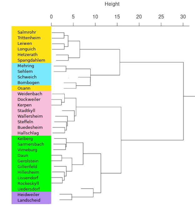
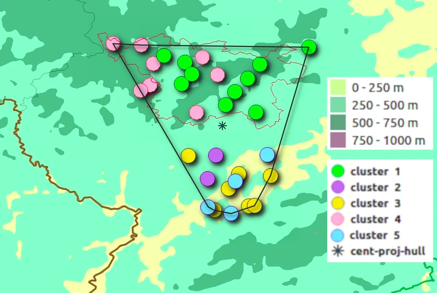
Clusters 1 and 4 occupy the high elevation areas in the north, while clusters 3 and 5 correspond to the Moselle valley in the south. Cluster 2 (Landscheid in the N and Heidweiler in the south) are more closely related with cluster 1 than with the geographically closer clusters 3 and 5.

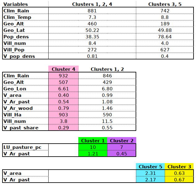
Table TYPOL – T01 – provides the averages of all the variables by cluster. It appears that cluster 1, 2 and 4 are characterised more by elevation and rainfall than by temperatrure. It also appears that what differentiates cluster 2 from all others is the reduced fingerprint of agriculture, a low wedding rate and large variability of population density, all compatible with relative isolation of the two localities.

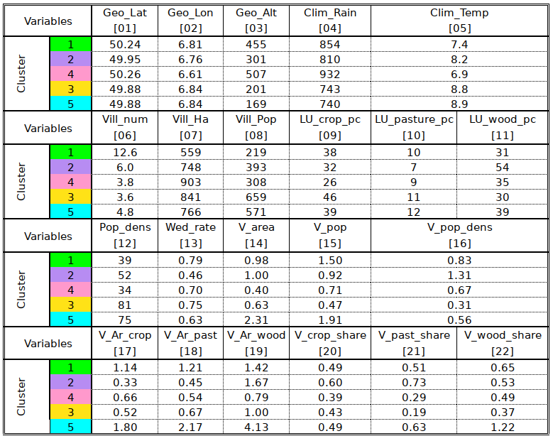
Clusters 3 and 5 feature low elevation and rainfall, large villages, high population density and low spatial variability((I.e. low variability among localities under the registry offices.)) as well as a larger share of land being dedicated to cropping (including gape vines) than in the northern areas.

Table TYPOL – T02 is based on an analysis of variance (ANOVA) provides a somewhat more objective approach to the statistical differences between clusters. The main divide between clusters 1, 2, 4 and 3, 5 is brought about by population and environmental differences. The separation between 4 and 1, 2 has to do with the homogeneity of land use village size. It is worth noting that 1 and 2 are more similar to each other than they are to cluster 4, which evidences the existence of a sparsely populated wet highland “high” Eifel type. Next to this we have the 1,2 clusters which are somewhat more favourable. Clusters 1 and 2 are separated, statistically (significantly so) by differences in the intensity of livestock husbandry and its spatial homogeneity. Spatial homogeneity (or inhomogeneity) is also what distinguishes clusters 3 and 5, in addition to several statistically non significant differences.

TYPOL.Addendum

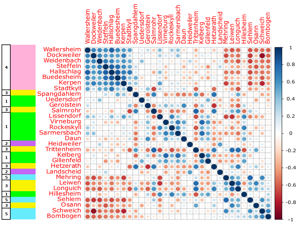
Figure TYPOL – F03 below illustrates the correlations between Registry offices based on the 22 standardised variables. It appears that cluster 4 is well defined for all the 8 Registry offices. Cluster 1 has a core of very similar Locations (Lissendorf to Daun) with Kelberg, Gillenfeld and especially Hillesheim being more losely associated with the core. Üdersdorf (cluster 1) has only weak associations (with Gillenfeld and Weidenbach, also cluster 1) which definitely puts it apart from cluster 2, as in TYPOL-F01. As to Osann (cluster 3), the correlation matrix confirms that its position close cluster 5 is also expressed by the 22 variables, in addition to the geographic vicinity.