This chapter deals with the relative origin of spouses, i.e. their origin (place of birth) relative to the Wedding registry office (RO; Standesamt) as well as their origin relative to each other. It is the twin-post to ABSOR, where it was shown that most spouses used to marry not far away from their birth places. RELOR is also related to chapter WEDNUM which characterises the inter-annual variations in the Number of weddings.
RELOR.1 Most people marry their neighbour!
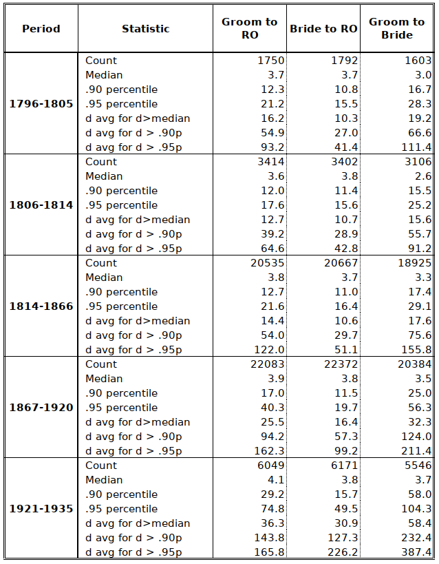
In addition to providing a general overview of the relative origin of spouses, Table RELOR-T01 provides some of the variables that will be presented for several other data sets and groupings in this chapter.
Count is the total number of grooms and brides for which relevant data are available, as well as the number of marriages for which both the origin of the groom and the birtplace of the bride could be determined (refer to chapter LOCATIONS for details). Average is the average distance in the three categories. Stdev is the standard deviation of the distance. It is noted that the values of Stdev are much larger than the average, which is a first indication of the fact that the small distance of about 10 km hides a more complex situation. Confidence stands for the confidence interval of the mean, i.e. 95% of distance values are includes in the interval Average-Confidence to Average+Confidence. Values are small due to the rather large number of observations. Reflecting the large Stdev, the coefficients of variation indicate the large inhomogeneity of the data. Skewness is a unitless statistic that describes the shape of the distribution of distance values. The rather large positive skew means that while most values are grouped at low distances, there is also a number of large distances that pull up the average1.
This appears again when comparing average and median. For the “Groom to RO” distance, the average amounts to 11.1 km, but 50% of the observations are smaller than 3.9 km and, logically, 50% are larger! The 0.9 percentile is the value such that 90% of distances are small (smaller than 14.8 km); 95% are smaller than 31.0 km. Yet, when computing the average of the 5% of values that are larger than 21 km, the more impressive average is found to be 147.2 km. Also consider that 5% of 53356 is 2783. Over the 135 years coverted by the Project, this is about 20 persones per year.
Altogether, according to table RELOR-T01, brides tend to be less mobile that their spouses, especially for the larger distances where husbands travel about 1.56 times the distances travelled by their wives. The median of the distance between the birthplaces of the spouses is just 3.4 km, which is to say that most people married their neighbour… except for 5% of them who travelled 207 km on average.
RELOR.2 How distances changed over time
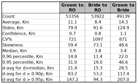
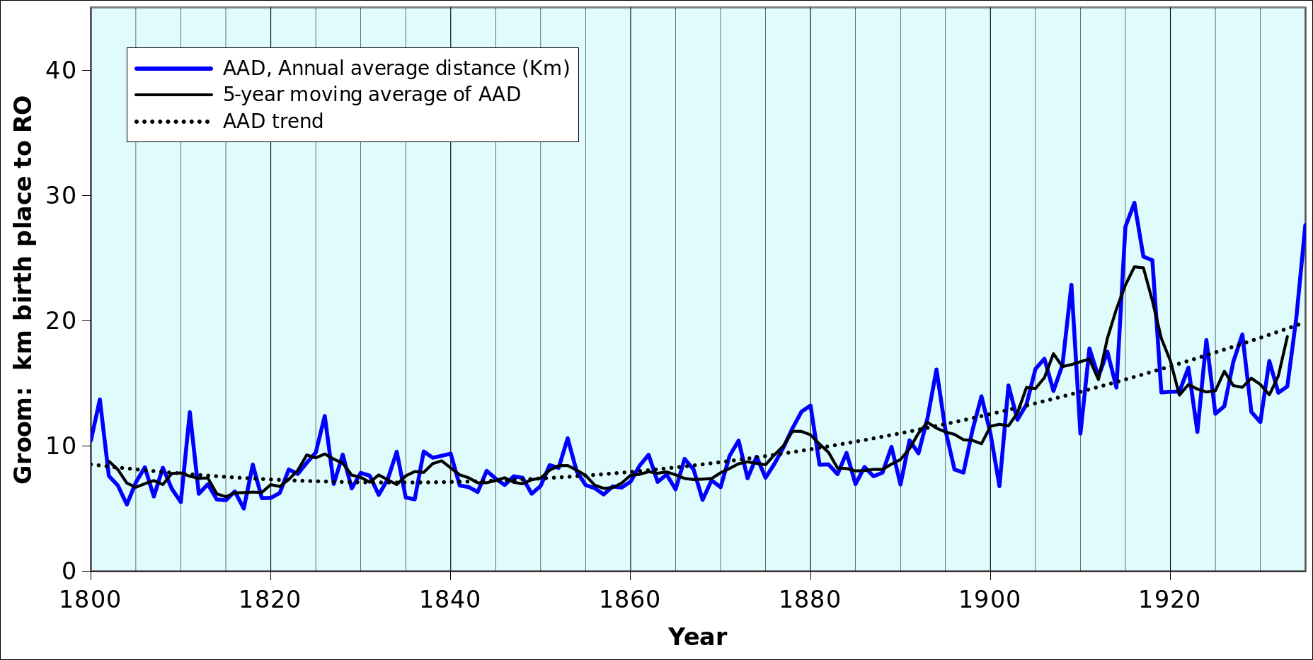
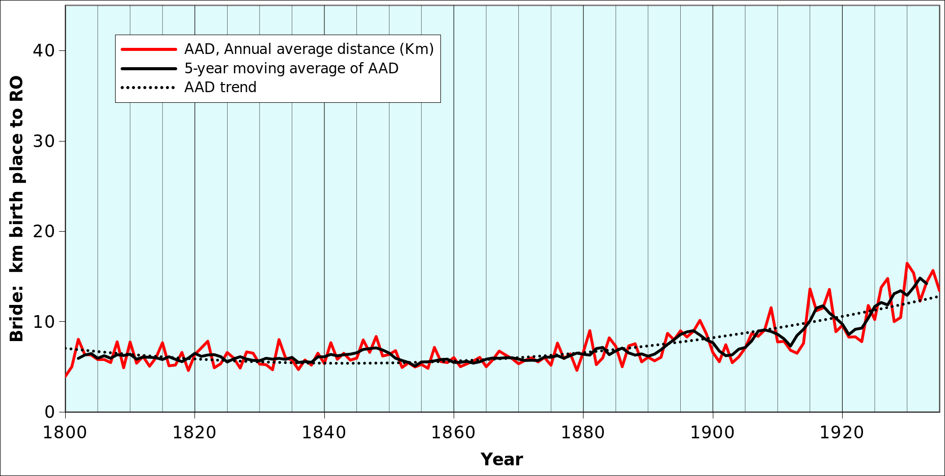
Figure RELOR-F01 illustrates how the distances varied over time. The graphs are based on data from which outliers were removed as very large distances markedly affect averages, pushing them towards high values. Refer to chapter METHODS.1 for full explanations.
The average number of available annual distances amounts to 361, 357 and 329, respectively, for the birthplace of the bride to RO, groom to RO et bride to groom places of birth. This is to say that, on average, each point in the graph is the average of more than 300 observations, which is a value of all respect by statistical standards! Minimum numbers of available distances mirror the number of weddings, as shown in more detail in chapter WEDNUM, and occur in during the first world war in 1915 (87, 79, 72) and just thereafter (1920, with 952, 921 and 854 values).
 |
 |
 |
A common behaviour of all curves is the “uneventful” pattern up to the end of the German confederation and the beginning of the German empire (refer to HIST.3 and Hist.4 in chapter HIST): low interannual variability of distances, stagnating values with an apparent minimum around 1840-1850 during the period of the German confederation, at the time of the 1848-49 revolutions2. For males, the beginning of the period, say up to 1820, was rather more “agitated” as may result from their willing or unwilling involvement with the turmoil brought about by Napoleonic adventurism.
The Franco-Prussian war of 1870, which covered in substance the second half of 1870 does not appear to have affected significantly the origin of spouses. Altogether, peaks for brides appear in 1846-47 in the wake of the potato blight, 1896-97, 1907-1908 and 1916 during WWI. Peaks for grooms do not coincide as they occur in 1801, 1815-16, 1811, 1826, 1879-80, 1894 and 1909.
The period after 1870 is marked by a significant increase of the distance over which spouses travelled for their marriage. The values increase from 10 km or below to about 20 km for males or just below 20 km for females in 1935, with significant interannual fluctuations from WWI and thereafter.
With the exception of “men from far away” marrying into the Project area during WWI3, it is not clear what may have triggered most of the peaks, all the more so because there is usually a time lag between people’s movements and their wedding4! Environmental variables and section HIST.3 indicate a wet period in the years leading up to 1880. To the contrary, years before 1900 were dry. The relative environmental abnormality may have been a factor, but with a low degree of confidence.
RELOR.3 Distance by historical periods
Table RELOR-T02 provides distance statistics according to the main historical periods described in chapter HIST. The increase of distance between birthplaces and Registry offices (RO) that was apparent in the graphs above is shows in the tables as well. In the pre-WWII period, the distance between the places of origin of brides and grooms increased very significantly to 387.4 km for the 5% of people who came from far away, more than double the distance in the pre-WWI period. In general, for the large distances, males travel about twice as far as females, with the notable exception of the 1921-35 period when 5% of women came from more than twice as far as their predecessors between 1867 and 1929 (226.2 km vs. 99.2 km). The observation does not affect men.
RELOR.4 Distance by cluster and by Registy office
Table RELOR-T03 below is yet another variant of RELOR-T01 and RELOR-T02, this time focusing on the clusters defined in chapter TYPOL and the registry offices themselves. When referrring to medians, throughout the period covered by the project, distances were largest in Cluster 1 (eastern Volcanic Eifel district) and smallest up to the Franco-Prussian war in Cluster 5 in the Moselle Valley. After the war, distances increased in the Moselle valley, but still remained smaller than in other areas.
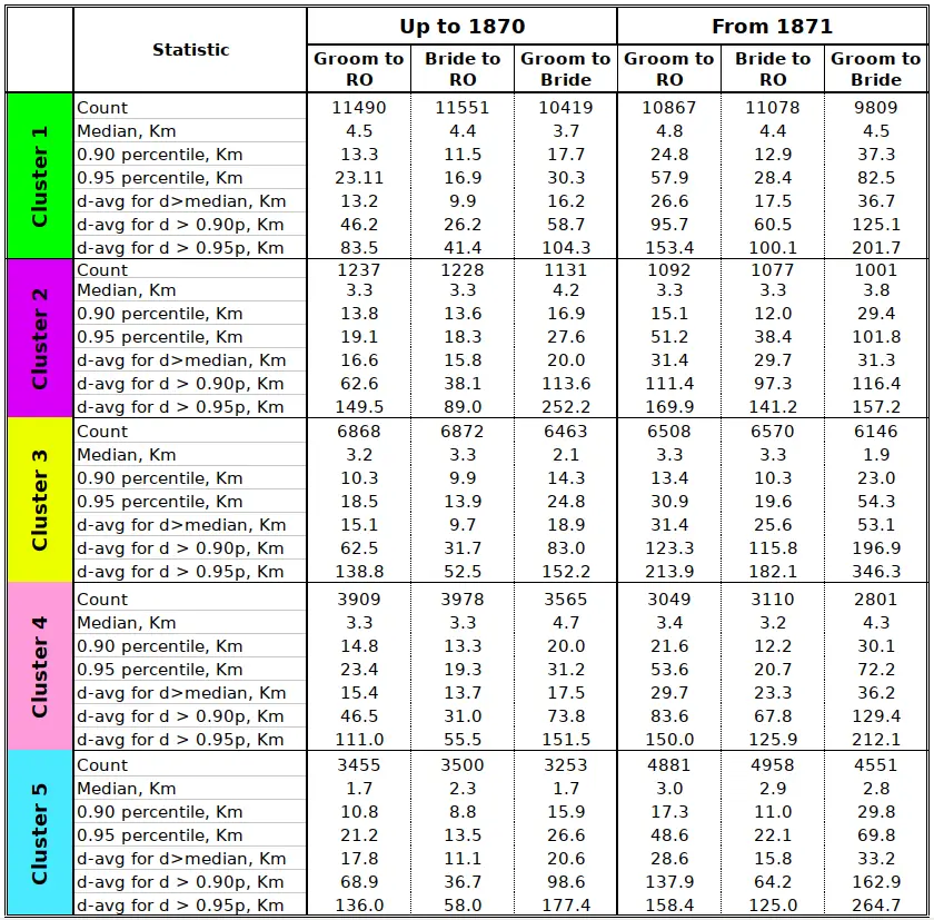
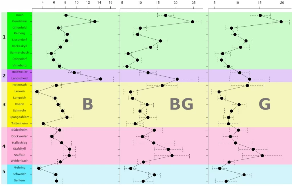
The most homogeneous cluster in terms of average distance for all categories (B, BG and G) appear to be the Moselle valley registry offices in Clusters 3 and 5. Cluster 4 could be mentioned as well for brides. Most other clusters are characterised by marked differences between ROs. In Cluster 1, for instance, Gerolstein displays values that are at least two times larger than those for Sarmersbach or Virneburg. Those differences persist when considering the confidence intervals. The largest absolute distance for brides is in Landscheid (Cluster 2). Interestingly, Cluster 2 is the one with the lowest wedding rates (refer to TYPOL-T01). For grooms, next to Gerolstein, we have Daun and Steffeln at distances close to 15 km.
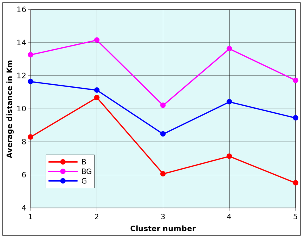
RELOR-F03 provides a simplified summary of the table (RELOR-T03) and figure (RELOR-F02) above showing generally low distances ìin Cluster 3, and especially for brides in Cluster 5, and larger values for grooms than for brides. The peak for brides in Cluster 2 (especially Landscheid) is also clearly visible. Note, incidentally, that the BG distance exceeds both B and G. This indicates that spouses come from different directions relative to the RO5.
RELOR.5 The mobility of local spouses
Table RELOR-T03 looks at the mobility of spouses as seen from the perspective of the registry offices. Note that this refers to the very locality of the RO (Standesamt) and does not include the localities of the Registry Office district (Standesamtbezirk)6.
The first two colums provide absolute numbers of spouses (whether brides or grooms) who originate in the RO locality, as well as the number who married locally. This includes spouses who married in other localities that are part of the database. Globally, about 85% (21553/25442) married locally7 .
The next four columns are expressed as percentages and provide the share of spouses who outmarried to one of the 35 localities in the Project area. As a rule, for the whole of table RELOR-T04, the sum of column 3 (e.g. 14 for DAUN) and the percentage of those who married locally (i.e. 689/805= 86%) reaches 100 %. In other words, the people born locally who married outside the Project area are very few and do not appear with the available data.
The next colum indicates the percentage of weddings with a local groom and those with a local bride. Remaining grooms and brides hail from other localities. These numbers provide an interesting indication about how “open to outsiders” or “closed to outsiders” the localities are. On average, clusters 1 and 2 used to be the most open8. The most closed cluster is 5, which seems somewhat paradoxical, considering that river valleys have often been corridors where people met. It may also be that the wealthier wine growers tended to intermarry to protect their assets!
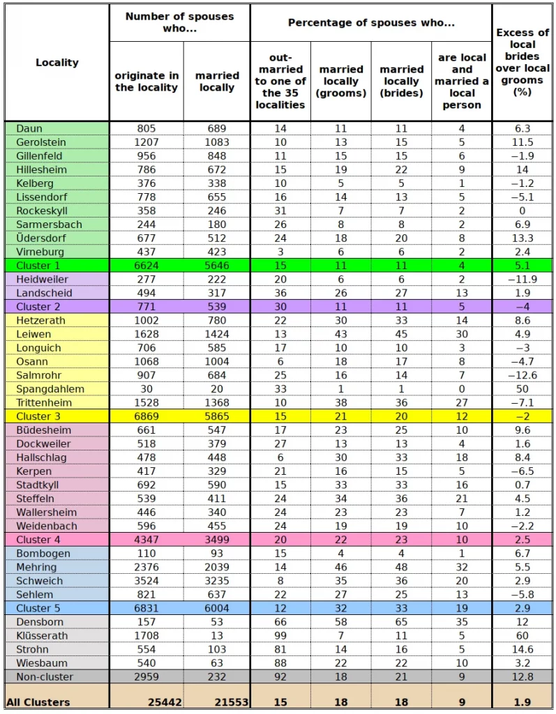
The smallest share of outsiders occurs in Hetzerath, Leiwen and Trittenheim (Cluster 3), Hallschlag, Stadtkyll and Steffelm (Cluster 4), Mehring and Schweich (Cluster 5). Among the localities with a complete record over time, the absolute records (more than 40% of marriages with local spouses) are in Leiwen and Mehring. In the same localities, both spouses are local in more than 30% of weddings.
The last variable, the Excess of local brides over local grooms (%) is computed as (NB-NG)/NG*100 % where NB is the number of local brides and NG is the number of local grooms. The lowest numbers occur in Clusters 2 and 3 (-4% and -2%, respectively). The lowest value (-12.6% in Salmrohr, Cluster 3; -11.9% in Heidweiler, Cluster 2) indicates that local women used to “import their husbands”. On the other hand, the Cluster that “imports” the largest share of its brides is Cluster 2 (5.1% on average), with Hillesheim, Üdersdorf and Gerolstein leading with 14.0%, 13.3% and 11.5%, respectively. If wives had to be “imported”, it is likely that many of them outmigrated, for instance to the cities located north of the Project Hull.
- A typical data set with a positive skew would be 0 0 0 0 0 0 0 0 0 100[↩]
- The observation may be due to a coincidence, altough the widespread insecurity may have kept people from exercising their Wanderlust.[↩]
- Peaks for Husbands three times larger than the peak for wives[↩]
- Even when considering that war changes some rules.[↩]
- If spouses came from exactly opposite directions, BG would be the sum of B and G. The bearings were actually computed alongside with the distances, but are not presented[↩]
- For instance, in 1885, the Standesamtbezirk of Daun included the localities of Boverath, Darscheid, Daun, Gemünden, Hörscheid, Mehren, Neunkirchen, Pützborn, Rengen, Schalkenmehren and Steinborn. Refer to DATA.8 for details.[↩]
- Remember that the total databse includes about 60000 weddings, i.e. 120000 spouses. Among those, 24442 originate in one of the Project localities. The others mostly come from nearby; refer, for instance, to ABSOR-F04a and ABSOR-F04b[↩]
- Although Landscheid, which is part of 2, is relatively closed.[↩]